Lecture

Figure: 1.1.4. Signal classification.
Signals are classified on the basis of essential features of the corresponding mathematical signal models. All signals are divided into two large groups: deterministic and random (Fig. 1.1.4).
Classification of deterministic signals. Usually, two classes of deterministic signals are distinguished: periodic and non-periodic.
Harmonic and polyharmonic signals are classified as periodic . For periodic signals, the general condition s (t) = s (t + kT) is fulfilled, where k = 1, 2, 3, ... is any integer, T is a period, which is a finite segment of the independent variable.
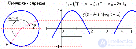
Harmonic signals (or sinusoidal) are described by the following formulas:
s (t) = A Ч sin (2 p f о t + f ) = A Ч sin ( w о t + f ),
s (t) = A Ч cos ( w о t + j ), (1.1.1)
where A, f o , w o , j, f are constants that can play the role of informational parameters of the signal: A is the signal amplitude, f o is the cyclic frequency in hertz, w o = 2 p f o is the angular frequency in radians, j and f are the initial phase angles in radians. The period of one oscillation T = 1 / f o = 2 p / w o . For j = f - p/ 2 sine and cosine functions describe the same signal. The frequency spectrum of the signal is represented by the amplitude and initial phase value of the frequency f about (at t = 0).
Polyharmonic signals make up the most widespread group of periodic signals and are described by the sum of harmonic oscillations:
s (t) =  A n sin (2 p f n t + j n ), (1.1.2)
or directly by the function s (t) = y (t ± kT p ), k = 1,2,3, ..., where T p is the period of one complete oscillation of the signal y (t), given in one period. The value f p = 1 / T p is called the fundamental vibration frequency. Polyharmonic signals are the sum of a certain constant component (f о = 0) and an arbitrary (in the limit - infinite) number of harmonic components with arbitrary values of the amplitudes A n and phases j n , with periods that are multiples of the period of the fundamental frequency f p . In other words, at the period of the fundamental frequency f p, which is equal to or multiples of the minimum harmonic frequency, is a multiple of the periods of all harmonics, which creates the frequency of signal repetition. The frequency spectrum of polyharmonic signals is discrete, and therefore the second common mathematical representation of signals is in the form of spectra (Fourier series).
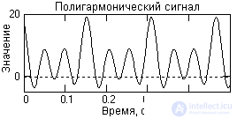
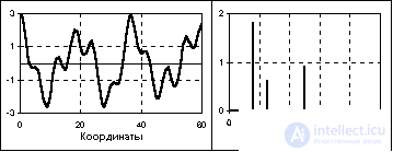
As an example, Fig. 1.1.6 shows a segment of the periodic signal function, which is obtained by summing the constant component (the frequency of the constant component is 0) and three harmonic oscillations with different values of the frequency and the initial phase of the oscillations. The mathematical description of the signal is given by the formula:
s (t) =  A k H cos (2 H pH f k H t + j k ),
where: A k = {5, 3, 4, 7} - amplitude of harmonics; f k = {0, 40, 80, 120} - frequency in hertz; j k = {0, -0.4, -0.6, -0.8} - initial phase angle of oscillations in radians; k = 0, 1, 2, 3. The fundamental frequency of the signal is 40 Hz.
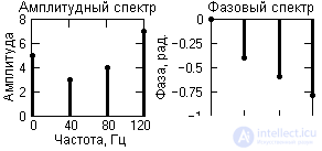
The frequency representation of this signal (signal spectrum) is shown in Fig. 1.1.7. Note that the frequency representation of the periodic signal s (t), limited by the number of spectrum harmonics, is only eight samples and is very compact compared to the time representation.
A periodic signal of any arbitrary shape can be represented as a sum of harmonic oscillations with frequencies that are multiples of the fundamental oscillation frequency f p = 1 / T p . To do this, it is enough to expand one signal period in a Fourier series in terms of the trigonometric functions of sine and cosine with a frequency step equal to the fundamental frequency of oscillations D f = f p :
s (t) =  (a k cos 2 p k D ft + b k sin 2 p k D ft), (1.1.3)
a o = (1 / T)  s (t) dt, a k = (2 / T) s (t) cos 2 p k D ft dt, (1.1.4)
b k = (2 / T) s (t) sin 2 p k D ft dt. (1.1.5)
The number of members of the Fourier series K = k max is usually limited by the maximum frequencies f max of harmonic components in the signals so that f max <K · f p . However, for signals with discontinuities and jumps, f max ® Ґ takes place , and the number of terms in the series is limited by the permissible error of approximation of the function s (t).
Single frequency cosine and sine harmonics can be combined and decomposed in a more compact form:
s (t) =  S k cos (2 p k D ft- j k ), (1.1.3 ')
S k =  , j k = argtg (b k / a k ). (1.1.6)
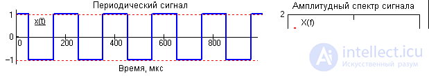
Figure: 1.1.8. Rectangular periodic signal (meander).
An example of representing a rectangular periodic signal (meander) in the form of an amplitude Fourier series in the frequency domain is shown in Fig. 1.1.8. The signal is even relative to t = 0, has no sine harmonics, all values of j k for a given signal model are equal to zero.
Informational parameters of a polyharmonic signal can be both certain features of the signal form (swing from minimum to maximum, extreme deviation from the mean, etc.), and the parameters of certain harmonics in this signal. So, for example, for rectangular pulses, the information parameters can be the pulse repetition period, pulse duration, pulse duty cycle (the ratio of the period to the duration) . When analyzing complex periodic signals, information parameters can also be:
- The current average value over a certain time, for example, over a period:
(1 / Т) s (t) dt.
- Constant component of one period:
(1 / Т) s (t) dt.
- Average rectified value:
(1 / T) | s (t) | dt.
- Mean square value:
 ...
...
Non-periodic signals include almost periodic and aperiodic signals. Frequency representation is also the main tool for their analysis.
Almost periodic signals are close in shape to polyharmonic. They also represent the sum of two or more harmonic signals (in the limit - to infinity), but not with multiples, but with arbitrary frequencies, the ratios of which (at least two frequencies at least) do not refer to rational numbers, as a result of which the fundamental period of the total oscillations is infinite great. So, for example, the sum of two harmonics with frequencies 2foand 3.5fogives a periodic signal (2 / 3.5 is a rational number) with a fundamental frequency of 0.5fo, in one period of which 4 periods of the first harmonic and 7 periods of the second will fit. But if the value of the second harmonic frequency is replaced by a close value offo  , then the signal goes into the category of non-periodic, since the ratio 2 / does not belong to the number of rational numbers. As a rule, almost periodic signals are generated by physical processes that are not related to each other. The mathematical display of signals is identical to polyharmonic signals (the sum of harmonics), and the frequency spectrum is also discrete.
Aperiodic signals make up the main group of non-periodic signals and are set by arbitrary functions of time. In fig. 1.1.10 shows an example of an aperiodic signal given by the formula on the interval (0,Ґ):
s (t) = exp (-a × t) - exp (-b × t),
where a and b are constants, in this case a = 0.15, b = 0.17.
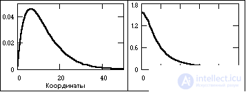

Figure: 1.1.10. Aperiodic signal and spectrum module. Figure: 1.1.11. Pulse signal and spectrum module.
Pulse signals also belong to aperiodic signals, which in radio engineering and in industries widely using it, are often considered as a separate class of signals. Pulses are signals, as a rule, of a certain and rather simple form, existing within finite time intervals. The signal shown in Fig. 1.1.11, refers to the pulse.
The frequency spectrum of aperiodic signals is continuous and can contain any harmonics in the frequency range [0, Ґ ]. To calculate it, the integral Fourier transform is used, which can be obtained by passing in formulas (1.1.3) from summation to integration as D f ® 0 and k D f ® f.
s (t) =  (a (f) cos 2 p ft + b (f) sin 2 p ft) df = S (f) cos (2 p ft- j (f)) df. (1.1.7)
a (f) = s (t) cos 2 p ft dt, b (f) = s (t) sin 2 p ft dt, (1.1.8)
S (f) =  , j (f) = argtg (b (f) / a (f)). (1.1.9)
The frequency functions a (f), b (f) and S (f) do not represent the amplitude values of the corresponding harmonics at certain frequencies, but the spectral density distributions of the amplitudes of these harmonics along the frequency scale. Formulas (1.1.8-1.1.9) are usually called formulas of direct Fourier transform, formulas (1.1.7) - inverse transformation.
If we are not interested in the behavior of the signal outside the area of its assignment [0, T], then this area can be perceived as one period of a periodic signal, i.e. the value of T is taken as the fundamental frequency of periodic oscillations, while for the frequency model of the signal, an expansion in Fourier series in the region of its assignment (1.1.3-1.1.6) can be applied.
In the class of impulse signals, a subclass of radio impulses is distinguished. An example of a radio pulse is shown in Fig. 1.1.12.
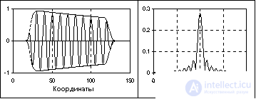
The radio pulse equation has the form :
s (t) = u (t) cos (2 p f o t + j o ).
where cos (2 p f o t + j o ) is the harmonic oscillation of the filling of the radio pulse, u (t) is the envelope of the radio pulse. The position of the main peak of the radio pulse spectrum on the frequency scale corresponds to the filling frequency f o , and its width is determined by the radio pulse duration. The longer the radio pulse duration, the smaller the width of the main frequency peak.
From an energetic standpoint, signals are divided into two classes: with limited (finite) energy and with infinite energy.
For signals with limited energy (otherwise - signals with an integrable square ), the following relation should be fulfilled:
 | s (t) | 2 dt <∞.
As a rule, this class of signals includes aperiodic and impulse signals that do not have breaks of the 2nd kind with a limited number of breaks of the 1st kind. Any periodic, polyharmonic and almost periodic signals, as well as signals with discontinuities and special points of the 2nd kind going to infinity, refer to signals with infinite energy. Special methods are used to analyze them.
Sometimes signals of finite duration are distinguished into a separate class, which differ from zero only on a limited interval of arguments (independent variables). Such signals are usually called finite signals .
Classification of random signals. A random signal is called a function of time, the values of which are not known in advance and can be predicted only with a certain probability.A random signal reflects a random physical phenomenon or a physical process, and the signal recorded in a single observation is not reproduced during repeated observations and cannot be described by an explicit mathematical dependence. When registering a random signal, only one of the possible variants (outcomes) of a random process is realized, and a sufficiently complete and accurate description of the process as a whole can be made only after repeated repetition of observations and calculating certain statistical characteristics of the ensemble of signal realizations. The main statistical characteristics of random signals are:
a) the distribution law of the probability of finding the signal value in a certain range of values;
b) spectral distribution of signal power.
Random signals are subdivided into stationary and non-stationary. Random stationary signals retain their statistical characteristics in sequential implementations of a random process. As for random non-stationary signals, their generally accepted classification does not exist. As a rule, various groups of signals are distinguished from them according to the features of their nonstationarity.

Comments
To leave a comment
Signal and linear systems theory
Terms: Signal and linear systems theory