Ways to normalize input data for non-network

Normalization of the input data is a process in which all input data goes through the process of "alignment", i.e. reduction to the interval [0,1] or [-1,1]. If you do not carry out normalization, the input data will have an additional effect on the neuron, which will lead to wrong decisions. In other words, how can we compare values ​​of different orders?

The need for normalization of data samples is due to the very nature of the used variables of neural network models. Being different in physical meaning, they can often vary greatly in absolute values. For example, a sample may contain both concentration, measured in tenths or hundredths of a percent, and pressure in hundreds of thousands of pascal. Data normalization allows bringing all used numerical values ​​of variables to the same area of ​​their change, which makes it possible to bring them together in one neural network model.

To perform data normalization, one needs to know precisely the limits of change in the values ​​of the corresponding variables (the minimum and maximum theoretically possible values). Then they will correspond to the limits of the normalization interval. When it is impossible to precisely set the limits of change of variables, they are set taking into account the minimum and maximum values ​​in the available data sample.

The most common way to normalize input and output variables is linear normalization .

Linear normalization

In general, the normalization formula looks like this:

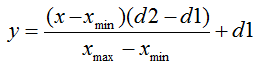
Where:

• - the value to be normalized;
• - the range of values ​​of x ;
• - the interval to which the value of x will be reduced.

Let me explain this with an example:

Let there be n input data from the interval [0,10], then = 0, and = 10. The data will lead to the interval [0,1], then = 0, and = 1. Now, substituting all the values ​​in the formula, we can calculate the normalized values ​​for any x from n input data.

In an abstract language, it looks like this:

  double d1 = 0.0;
 double d2 = 1.0;
 double x_min = iMA_buf [min (iMA_buf)];
 double x_max = iMA_buf [max (iMA_buf)]; 

 for (int i = 0; i <ArraySize (iMA_buf); i ++)
 {
 inputs [i] = (((iMA_buf [i] -x_min) * (d2-d1)) / (x_max-x_min)) + d1;
 } 

First, we specify the extreme values ​​for the output value, then we get the minimum and maximum values ​​of the indicator (copying data from the indicator is omitted, but for example there may be 10 last values). In the last step, we will perform a normalization of each input element in the cycle (indicator values ​​on various bars) and save it into an array for further work with it.

We adopt the following notation:

- xik , yjk - i -th input and j -th output values ​​of the k -th example of the original sample in the traditional units of measurement adopted in the problem being solved;

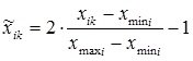
- - the corresponding normalized input and output values;

- N is the number of examples of the training sample.

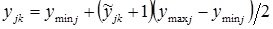
Then the transition from traditional to normalized units of measurement and back using the method of linear normalization is carried out using the following calculated ratios:

- with normalization and denormalization within [0, 1]:

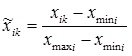; (one)

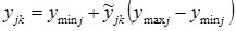; (2)

- with normalization and denormalization within [–1, 1]:

;

,

Where

;

.

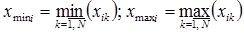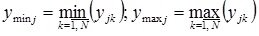If the training sample contains no examples with potentially smaller or larger output values, you can set the width of the extrapolation corridor for left, right, or both boundaries in fractions of the length of the entire initial interval of change of a variable, usually not more than 10% of it. In this case, there is a transition from the actual boundaries of the training sample to the hypothetical:

.

Nonlinear normalization

One of the methods of nonlinear normalization is using sigmoid logistic function or hyperbolic tangent. The transition from traditional to normalized units of measurement and back in this case is carried out as follows:

- with normalization and denormalization within [0, 1]:

;

,

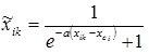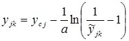where xc i, yc j are the centers of normalized intervals for changing the input and output variables:

;

- with normalization and denormalization within [–1, 1]:

;

.

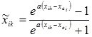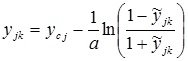The parameter a affects the degree of nonlinearity of the change in the variable in the normalized interval. In addition, when using values ​​of a <0.5, there is no need to additionally specify the width of the extrapolation corridor.

Consider comparing methods of linear and nonlinear normalization. In fig. 1 shows the graphs of the normalization of the input variable for the limits [–1; one]. For nonlinear normalization, using the function of the hyperbolic tangent, the value of the parameter a = 1.0 is taken. It should be noted that the coincidence of the normalized value in both cases takes place only at the point corresponding to the center of the normalized interval.

Fig. 1. Comparison of linear and nonlinear normalization functions

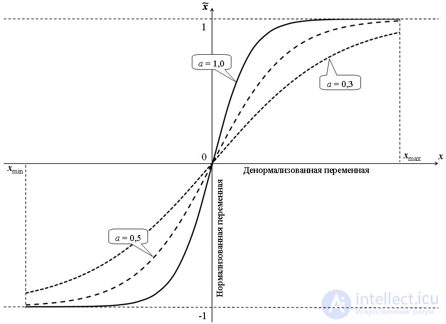
Fig. 2. The effect of the parameter on the graph of the nonlinear normalization function

In fig. 2 shows cases of nonlinear normalization within [0; 1] using the hyperbolic tangent function with parameters a equal to, respectively, 0.3, 0.5, 1.0. Obviously, the smaller the value of the parameter a , the more hollow the normalized dependence looks and the greater the width of the extrapolation corridor.