Lecture
In this article we will talk about Elman's recurrent neural network [1], which is also called the Simple Recurrent Neural Network (Simple RNN, SRN).
There are actual data processing problems, when solving which we encounter not individual objects but their sequences, i.e. the order of objects plays a significant role in the task. For example, this is a speech recognition problem, where we are dealing with sequences of sounds or some natural-text processing tasks [2], where we are dealing with sequences of words.
To solve such problems, you can use recurrent neural networks, which in the process can save information about their previous states. Next, we consider the principles of operation of such networks on the example of Elman's recurrent network [1].
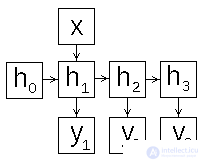
Artificial neural network Ellman [1], also known as Simple Recurrent Neural Network, consists of three layers - input (distribution) layer, hidden and output (processing) layers. In this case, the hidden layer has a feedback on itself. Figure 1 presents the scheme of the neural network of Elman.

Figure 1: Elman's neural network diagram
In contrast to the normal network of direct distribution [3], the input image of the recurrent network is not one vector but the sequence of vectors { x ( 1 ) , ... x ( n ) } {x (1), ... x (n)} , the vectors of the input image in a given order are fed to the input, while the new state of the hidden layer depends on its previous states. The Elman network can be described by the following relations.
h ( t ) = f ( V ⋅ x ( t ) + U ⋅ h ( t - 1 ) + b h ) h ( t ) = f ( V ⋅ x ( t ) + U ⋅ h ( t − 1) + bh )
y ( t ) = g ( W ⋅ h ( t ) + b y ) y ( t ) = g ( W ⋅ h (t) + by)
here
x ( t ) x (t) - input vector number t t ,
h ( t ) h (t) - the state of the hidden layer for the input x ( t ) x (t) ( h ( 0 ) = 0 h (0) = 0 ),
y ( t ) y (t) - network output for input x ( t ) x (t) ,
U u - weight matrix distribution layer
W W - weight (square) matrix of feedbacks of the hidden layer,
b h bh - vector of shifts of the hidden layer,
V v - weight matrix of the output layer,
b y by - vector of shifts of the output layer
f f - hidden layer activation function
g g - activation function of the output layer
In this case, there are various schemes of the network, which we will discuss in the next section.
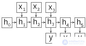
Depending on how to form the input and output of the recurrent network, you can set the scheme of its operation in different ways. Consider this question in more detail, for this we expand the scheme of the recurrent network in time (Fig. 2).
 |
 |
 |
| a) | b) | c) |
 |
| d) |
Figure 2: recurrent neural network operation patterns
We list the possible ways of organizing the work of a recurrent network [4,5].
Next we look at the method of learning network Emana.
In this section, we describe the method of learning the recurrent Ellman network using the many-to-one scheme (Fig. 2a), for implementing a classifier of objects defined by sequences of vectors. For learning of the Elman network, the same gradient methods [3] are used as for ordinary networks of direct propagation, but with certain modifications, to correctly calculate the gradient of the error function. It is calculated using a modified back-propagation method [3], which is called Backpropagation through time (back-propagation method with network expansion in time, BPTT) [6]. The idea of the method is to expand the sequence, turning the recurrent network into a “normal” one (Fig. 2a). As in the backpropagation method for forward propagation networks [3], the process of calculating the gradient (changing weights) occurs in the following three steps.
Consider these steps in more detail.
1. Direct passage: for each vector of the sequence { x ( 1 ) , ... x ( n ) } {x (1), ... x (n)} :
calculate the states of the hidden layer { s ( 1 ) , ... s ( n ) } {s (1), ... s (n)} and exits of the hidden layer
{ h ( 1 ) , ... h ( n ) } {h (1), ... h (n)}
s ( t ) = V x ( t ) + U h ( t − 1 ) + a s ( t ) = V x ( t ) + U h ( t − 1) + a
h ( t ) = f ( s ( t ) ) h (t) = f (s (t))
calculate network output y y
y ( n ) = g ( W ⋅ h ( n ) + b ) y ( n ) = g ( W ⋅ h (n) + b)
2. Back pass: we calculate the error of the output layer δ o δo
δ o = y - d δo = y − d
calculate the error of the hidden layer in the final state δ h ( n ) δh (n)
δ h ( n ) = W T ⋅ δ o ⊙ f ′ ( s ( n ) ) δh (n) = WT⋅δo⊙ f ′ (s (n))
calculate hidden layer errors in intermediate states δ h ( t ) δh (t) ( t = 1 , ... n t = 1, ... n )
δ h ( t ) = U T ⋅ δ h ( t + 1 ) ⊙ f ′ ( s ( n ) ) δ h ( t ) = U T ⋅ δ h ( t + 1 ) f ′ (s (n))
3. Calculate the change in weights:
) T ΔW = δo⋅ (h (n)) T
Δ b y = ∑ δ o Δby = ∑ δo
) T ΔV = ∑tδh (t) ⋅ (x (t)) T
) T ΔU = ∑tδh (t) ⋅ (h (t − 1)) T
Δ b h = ∑ ∑ t δ h ( t ) Δbh = ∑∑ tδh (t)
Having found a method for calculating the gradient of the error function, then we can apply one of the modifications of the gradient descent method, which are described in detail in [3].
This section presents the implementation of the Elman recurrent network according to the many-to-one scheme (Fig. 2a), the activation of the hidden layer - the hyperbolic tangent (tanh), the activation of the output layer (softmax), the error function - the average cross-entropy. Learning data is randomly generated.
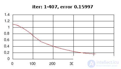
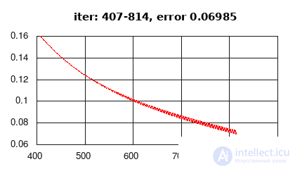
Figure 3: history of the change in learning error

Comments
To leave a comment
Computational Intelligence
Terms: Computational Intelligence