Lecture
A neural network is a sequence of neurons connected by synapses. The structure of the neural network came into the world of programming straight from biology. Thanks to this structure, the machine acquires the ability to analyze and even memorize various information. Neural networks are also able not only to analyze incoming information, but also to reproduce it from its memory. Interested be sure to watch 2 videos from TED Talks: Video 1, Video 2). In other words, the neural network is a machine interpretation of the human brain, in which there are millions of neurons transmitting information in the form of electrical impulses.
For now, we will consider examples at the most basic type of neural networks - this is a network of direct distribution (hereinafter referred to as SPR). Also in subsequent articles I will introduce more concepts and tell you about recurrent neural networks. AB, as the name implies, is a network with a series connection of neural layers, information in it always goes only in one direction.
Neural networks are used to solve complex problems that require analytical calculations similar to those of the human brain. The most common applications of neural networks are:
Classification - the distribution of data by parameters. For example, a set of people is given at the entrance and it is necessary to decide which of them to give a loan and who does not. This work can be done by a neural network, analyzing such information as: age, solvency, credit history, and so on.
Prediction - the ability to predict the next step. For example, rising or falling stocks, based on the situation on the stock market.
Recognition is currently the widest application of neural networks. Used by Google when you are looking for a photo or in the camera phones, when it determines the position of your face and highlights it, and more.
Now, in order to understand how neural networks work, let's take a look at its components and their parameters.
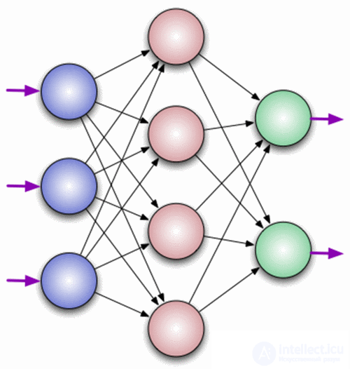
A neuron is a computational unit that receives information, performs simple calculations on it, and passes it on. They are divided into three main types: input (blue), hidden (red) and output (green). There is also a displacement neuron and a context neuron which we will discuss in the next article. In the case when the neural network consists of a large number of neurons, the term layer is introduced. Accordingly, there is an input layer that receives information, n hidden layers (usually no more than 3 of them) that process it and an output layer that displays the result. Each of the neurons has 2 basic parameters: input data (input data) and output data (output data). In the case of an input neuron: input = output. In the others, the total information of all neurons from the previous layer gets into the input field, after which it is normalized using the activation function (for now just present it to f (x)) and enters the output field.
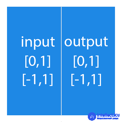
It is important to remember that neurons operate with numbers in the range [0,1] or [-1,1]. And what, you ask, then handle the numbers that fall outside this range? At this stage, the easiest answer is to divide 1 by this number. This process is called normalization, and it is very often used in neural networks. More on this later.
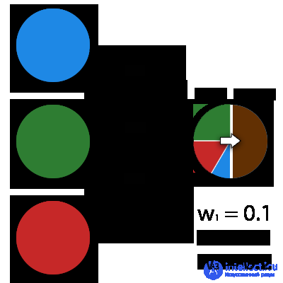
A synapse is the connection between two neurons. Synapses have 1 parameter - weight. Thanks to him, the input information changes when it is transmitted from one neuron to another. Suppose there are 3 neurons that transmit information to the following. Then we have 3 weights corresponding to each of these neurons. In that neuron, whose weight will be greater, that information will be dominant in the next neuron (for example, color mixing). In fact, a set of weights of a neural network or a matrix of weights is a kind of brain of the whole system. Thanks to these weights, the input information is processed and turned into a result.
It is important to remember that during the initialization of the neural network, the weights are placed randomly.
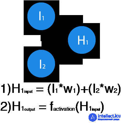
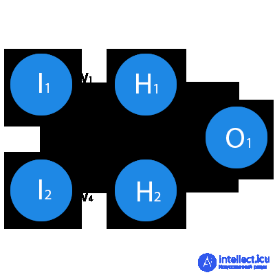
In this example, a part of the neural network is depicted, where the letters I denote the input neurons, the letter H represents the hidden neuron, and the letter w denotes weights. From the formula it is clear that the input information is the sum of all the input data multiplied by the corresponding weight. Then we give input 1 and 0. Let w1 = 0.4 and w2 = 0.7. The input data of the H1 neuron will be as follows: 1 * 0.4 + 0 * 0.7 = 0.4. Now that we have the input data, we can get the output by substituting the input value into the activation function (more on this later). Now that we have the output, we pass it on. And so, we repeat for all layers until we reach the output neuron. By launching such a network for the first time, we will see that the answer is far from correct, because the network is not trained. To improve the results we will train it. But before we learn how to do this, let's introduce a few terms and properties of the neural network.
The activation function is a way to normalize the input data (we already talked about this earlier). That is, if you have a large number at the entrance, by passing it through the activation function, you will get an exit in the range you need. There are a lot of activation functions, so we will consider the most basic ones: Linear, Sigmoid (Logistic) and Hyperbolic tangent. Their main differences are the range of values.
Linear function
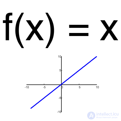
This function is almost never used, except when it is necessary to test a neural network or transmit a value without transformation.
Sigmoid
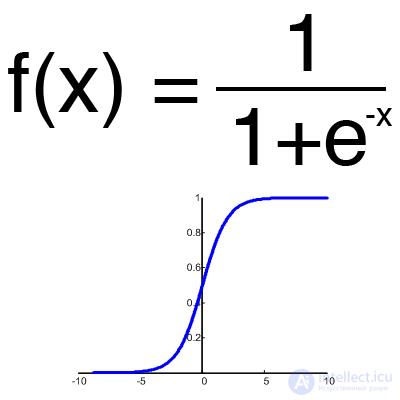
This is the most common activation function, its range of values is [0,1]. It shows the majority of examples in the network, it is also sometimes called the logistic function. Accordingly, if in your case there are negative values (for example, stocks can go not only up, but also down), then you need a function that captures negative values.
Hyperbolic tangent

It makes sense to use a hyperbolic tangent, only when your values can be both negative and positive, since the range of the function is [-1,1]. It is impractical to use this function only with positive values, since this will significantly worsen the results of your neural network.
A training set is a sequence of data with which a neural network operates. In our case, the exclusive or (xor) we have only 4 different outcomes, that is, we will have 4 training sets: 0xor0 = 0, 0xor1 = 1, 1xor0 = 1.1xor1 = 0.
This is a kind of counter that increases each time a neural network passes one training set. In other words, this is the total number of training sets passed by the neural network.
When the neural network is initialized, this value is set to 0 and has a ceiling that is set manually. The greater the era, the better the network is trained and, accordingly, its result. The era increases each time we go through the entire set of training sets, in our case, 4 sets or 4 iterations.

It is important not to confuse the iteration with the epoch and to understand the sequence of their increment. N first
times the iteration increases, and then the era and not vice versa. In other words, you cannot first train a neural network only on one set, then on another, and so on. You need to train each set once per era. So, you can avoid computation errors.
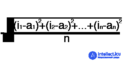
Error is a percentage value that reflects the discrepancy between the expected and received responses. A mistake is formed every era and should go into decline. If this does not happen, then you are doing something wrong. The error can be calculated in different ways, but we will consider only three main methods: Mean Squared Error (hereinafter MSE), Root MSE and Arctan. There is no restriction on use, as in the activation function, and you are free to choose any method that will bring you the best result. One has only to consider that each method counts errors in different ways. In Arctan, the error will almost always be greater, since it works on the principle: the greater the difference, the greater the error. Root MSE will have the smallest error, which is why, most often, MSE is used, which maintains a balance in the error calculation.
MSE

Root MSE
Arctan
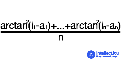
The principle of error counting is the same in all cases. For each set, we consider an error, taking away from the ideal answer, received. Next, either squaring or calculating the square tangent from this difference, after which the resulting number is divided by the number of sets.
Now, to test yourself, calculate the result of the given neural network using sigmoid and its error using MSE.
Data: I1 = 1, I2 = 0, w1 = 0.45, w2 = 0.78, w3 = -0.12, w4 = 0.13, w5 = 1.5, w6 = -2.3.
Decision
H1input = 1 * 0.45 + 0 * -0.12 = 0.45
H1output = sigmoid (0.45) = 0.61
H2input = 1 * 0.78 + 0 * 0.13 = 0.78
H2output = sigmoid (0.78) = 0.69
O1input = 0.61 * 1.5 + 0.69 * -2.3 = -0.672
O1output = sigmoid (-0.672) = 0.33
O1ideal = 1 (0xor1 = 1)
Error = ((1-0.33) ^ 2) /1=0.45
The result is 0.33, an error is 45%.
Thank you very much for your attention! I hope that this article was able to help you in the study of neural networks. In the next article, I will talk about displacement neurons and how to train a neural network using the back propagation method and gradient descent.
Now, consider the ways of teaching / training neural networks (in particular, the method of reverse propagation) and if for some reason you have not read the first part, I strongly recommend starting with it. In the process of writing this article, I also wanted to talk about other types of neural networks and training methods, however, starting to write about them, I realized that this would go against my method of presentation. I understand that you are not eager to get as much information as possible, however these topics are very extensive and require detailed analysis, and my main task is not to write another article with a superficial explanation, but to bring you every aspect of the topic touched and make the article as easy as possible. mastering. I hasten to upset the fans of "cool", since I still will not resort to the use of a programming language and will explain everything "on the fingers." Enough entry, let's now continue to study neural networks.
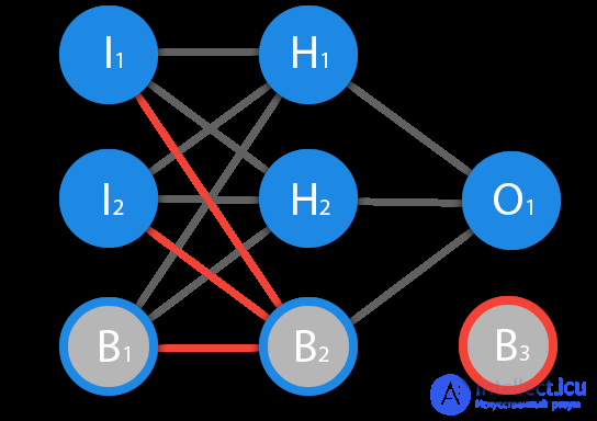
Before we begin our main topic, we must introduce the concept of another type of neuron - the displacement neuron. The displacement neuron or bias neuron is the third type of neuron used in most neural networks. The peculiarity of this type of neuron is that its input and output always equal 1 and they never have input synapses. Neurons of displacement can either be present in the neural network one by one on the layer, or completely absent, 50/50 cannot be (red on the diagram indicates weights and neurons that cannot be placed). Connections in neurons of displacement are the same as in normal neurons - with all neurons of the next level, except that there can be no synapses between two bias neurons. Consequently, they can be placed on the input layer and all hidden layers, but not on the output layer, since they simply will not have anything to form a connection with.
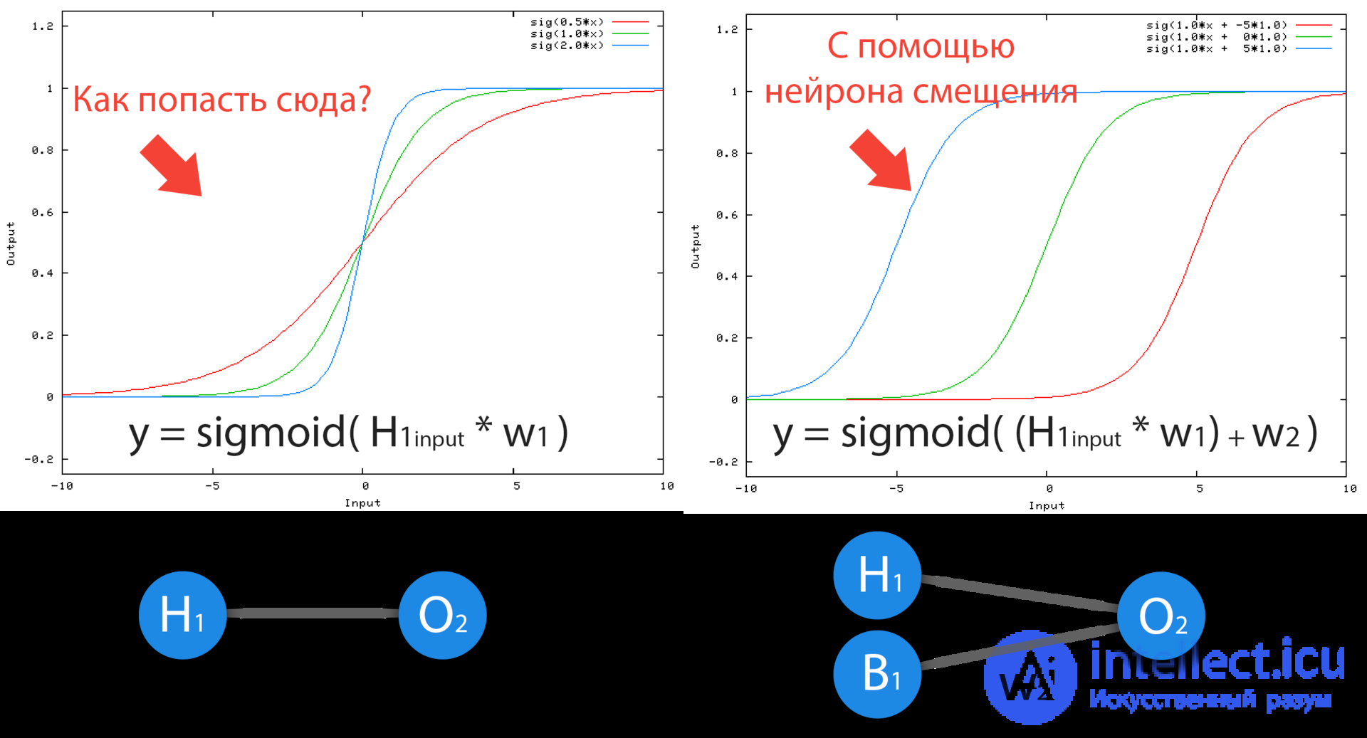
Neuron bias is needed in order to be able to get the output by shifting the graph of the activation function to the right or left. If this sounds confusing, let's look at a simple example where there is one input neuron and one output neuron. Then it can be established that the O2 output will be equal to the H1 input multiplied by its weight and passed through the activation function (the formula in the photo on the left). In our particular case, we will use sigmoid.
From the school course of mathematics, we know that if we take the function y = ax + b and change the values of “a” for it, the slope of the function will change (the colors of the lines in the graph on the left), and if we change the “b”, we will shift function to the right or left (colors of the lines in the graph to the right) So “a” is the weight of H1, and “b” is the weight of the displacement neuron B1. This is a rough example, but this is how it works (if you look at the activation function on the right of the image, you will notice a very strong similarity between the formulas). That is, when during training, we adjust the weights of hidden and output neurons, we change the slope of the activation function. However, the regulation of the weight of the neurons of displacement can give us the opportunity to shift the activation function along the X axis and capture new areas. In other words, if the point responsible for your decision is located, as shown in the graph on the left, then your NA will never be able to solve the problem without using displacement neurons. Therefore, you rarely find neural networks without neuronal displacement.
Also, displacement neurons help in the case when all input neurons receive input 0 and no matter what weight they have, they will all pass to the next layer 0, but not in the presence of a displacement neuron. The presence or absence of displacement neurons is a hyperparameter (more on this later). In a word, you yourself have to decide whether you need to use displacement neurons or not, driving out the NA with mixing neurons and without them and comparing the results.
It is IMPORTANT to know that sometimes the circuits do not indicate displacement neurons, but simply take their weights into account when calculating the input value for example:
input = H1 * w1 + H2 * w2 + b3
b3 = bias * w3
Since its output is always 1, you can simply imagine that we have an additional synapse with weight and add this weight to the sum without mentioning the neuron itself.
The answer is simple - you need to train her. However, no matter how simple the answer, its implementation in terms of simplicity, leaves much to be desired. There are several methods of teaching NA and I will highlight 3, in my opinion, the most interesting:
About Rprop and GA will be discussed in other articles, and now we will look at the basis of the basics - the backpropagation method that uses the gradient descent algorithm.
This is a way to find a local minimum or maximum of a function by moving along a gradient. If you understand the essence of the gradient descent, then you should not have any questions while using the back propagation method. To begin with, let's see what the gradient is and where it is present in our NA. Let's build a graph where the x-axis will be the weight values of the neuron (w) and the y-axis is the error corresponding to this weight (e).
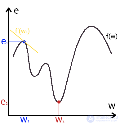
Looking at this graph, we understand that the graph function f (w) is the dependence of the error on the selected weight. On this chart, we are interested in the global minimum - a point (w2, e2) or, in other words, the place where the graph comes closest to the x-axis. This point will mean that choosing the weight w2 we get the smallest error - e2 and as a result, the best result possible.This is a yellow background in the graph. Find out the global minimum.
So what is this gradient? A gradient is a vector that determines the steepness of the slope and indicates its direction relative to any of the points on the surface or graph. To find the gradient you need to take the derivative of the graph at a given point (as shown in the graph). Moving in the direction of this gradient, we will smoothly roll down to the lowland. Now imagine that a mistake is a skier, and a graph of a function is a mountain. Accordingly, if the error is 100%, then the skier is at the very top of the mountain, and if the error is 0%, then in the lowland. Like all skiers, the error tends to go down as quickly as possible and reduce its value. In the final case, we should have the following result:
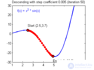
Imagine that a skier is thrown onto a mountain with a helicopter. How high or low depends on the case (in the same way as in a neural network when we initialize weights are placed in a random order). Let's say the error is 90% and this is our point of reference. Now the skier needs to go down using the gradient. On the way down, at each point we will calculate the gradient, which will show us the direction of descent and, when the slope changes, adjust it. If the slope is straight, then after the nth number of such actions we will reach the lowlands. But in most cases the slope (graph of the function) will be wavy and our skier will face a very serious problem - a local minimum. I think everyone knows what a local and global minimum of function is, to refresh your memory, here is an example. Hitting the local minimum is fraught withthat our skier will remain forever in this lowland and never slide down the mountain, therefore we can never get the right answer. But we can avoid this by equipping our skier with a jetpack called the moment (momentum). Here is a brief illustration of the moment:

As you may have guessed, this backpack will give the skier the necessary acceleration to overcome the hill that keeps us at a local minimum, but there is one BUT here. Imagine that we set a certain value to the moment parameter and easily managed to overcome all local minima and get to the global minimum. Since we cannot simply turn off the jet pack, we can slip through the global minimum if there are lowlands next to it. In the final case, this is not so important, because sooner or later we will still return back to the global minimum, but it is worth remembering that the greater the moment, the greater the scope with which the skier will ride through the lowlands. Together with the moment, such a parameter as the learning rate (learning rate) is also used in the back propagation method. How many will surely thinkthe greater the learning speed, the faster we will train the neural network. Not.The speed of learning, as well as the moment, is a hyperparameter - a quantity that is selected by trial and error. The speed of learning can be directly linked to the speed of a skier, and you can say with confidence that you will continue to walk quieter. However, there are also certain aspects here, because if we do not give the skier speed at all, he will not go anywhere at all, and if we give a small speed, the travel time can take a very, very long period of time. What then happens if we give too much speed?
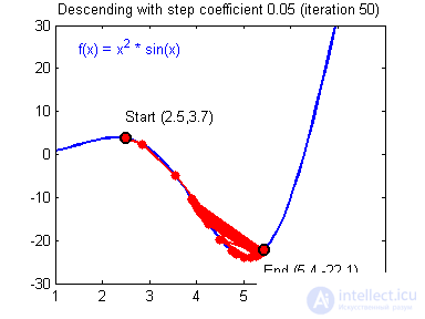
As you can see, nothing good. A skier will begin to slip down the wrong path and maybe even in a different direction, which, as you understand, only keeps us away from finding the right answer. Therefore, in all these parameters, it is necessary to find a middle ground to avoid non-convergence of the NA (more on that later).
So we have come to the point where we can discuss how to make it all the same so that your NA can properly learn and make the right decisions. Very good MOR visualized on this gif:

And now let's take a detailed look at each stage. If you remember that in the previous article we considered the output of the National Assembly. In another it is called forward transmission (Forward pass), that is, we consistently transmit information from the input neurons to the output. After that, we calculate the error and based on it we make a reverse transmission, which is to consistently change the weights of the neural network, starting with the weights of the output neuron. The value of weights will change in the direction that will give us the best result. In my calculations, I will use the delta method, as this is the easiest and most understandable way. Also, I will use the stochastic method of updating the weights (more on that later).
Now let's continue from where we completed the calculations in the previous article.
Task data from previous article
Data: I1 = 1, I2 = 0, w1 = 0.45, w2 = 0.78, w3 = -0.12, w4 = 0.13, w5 = 1.5, w6 = -2.3.
H1input = 1 * 0.45 + 0 * -0.12 = 0.45
H1output = sigmoid (0.45) = 0.61
H2input = 1 * 0.78 + 0 * 0.13 = 0.78
H2output = sigmoid (0.78) = 0.69
O1input = 0.61 * 1.5 + 0.69 * -2.3 = -0.672
O1output = sigmoid (-0.672) = 0.33
O1ideal = 1 (0xor1 = 1)
Error = ((1-0.33) ^ 2) /1=0.45
The result is 0.33, the error is 45%.
Since we have already calculated the result of the NA and its error, we can immediately proceed to the MPA. As I mentioned earlier, the algorithm always starts with the output neuron. In this case, let's calculate the value of δ (delta) for it by the formula 1.
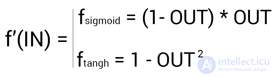
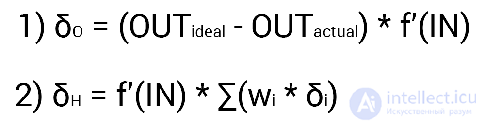 Since the output neuron has no outgoing synapses, we will use the first formula (δ output), therefore for the hidden neurons we will already take the second formula (δ hidden). Everything is quite simple here: we consider the difference between the desired and the obtained result and multiply by the derivative of the activation function of the input value of the neuron. Before proceeding with the calculations, I want to draw your attention to the derivative. First of all, as it has probably already become clear, with MPA, only those activation functions that can be differentiated should be used. Secondly, in order not to do extra calculations, the derivative formula can be replaced with a more friendly and simple formula of the form:
Thus, our calculations for the O1 point will look like this.
Decision
O1output = 0.33
O1ideal = 1
Error = 0.45
δO1 = (1 — 0.33) * ( (1 — 0.33) * 0.33 ) = 0.148
This completes the calculations for the O1 neuron. Remember that after calculating the neuron delta, we are obliged to immediately update the weights of all outgoing synapses of this neuron. Since they are not in the case of O1, we go to the neurons of the hidden level and do the same for the exception that the delta calculation formula is now our second and its essence is to multiply the derivative of the activation function from the input value by the sum of the products of all outgoing weights and delta of the neuron with which this synapse is connected. But why are the formulas different? The fact is that the whole essence of the MPA is to spread the error of the output neurons to all the weights of the NA. The error can be calculated only at the output level, as we have already done, we also calculated the delta in which this error already exists.Consequently, now instead of an error we will use a delta which will be transmitted from the neuron to the neuron. In this case, let's find the delta for H1:
Decision
H1output = 0.61
w5 = 1.5
δO1 = 0.148
δH1 = ((1 - 0.61) * 0.61) * (1.5 * 0.148) = 0.053
Now we need to find a gradient for each outgoing synapse. Here they usually insert a 3-story fraction with a bunch of derivatives and other mathematical hell, but that's the beauty of using the delta calculation method, because ultimately your gradient formula will look like this:

Here point A is the point at the beginning of the synapse, and point B at the end of the synapse. Thus, we can calculate the w5 gradient as follows:
Decision
H1output = 0.61
δO1 = 0.148
GRADw5 = 0.61 * 0.148 = 0.09
Now we have all the necessary data to update the weight of w5 and we will do this thanks to the MPA function which calculates the value by which this or that weight needs to be changed and it looks like this: We

strongly recommend that you do not ignore the second part of the expression and use the moment as you will avoid problems with the local minimum.
Here we see 2 constants about which we already spoke, when we considered the gradient descent algorithm: E (epsilon) - learning rate, α (alpha) - moment. Translating the formula into words we get: the change in the weight of the synapse is equal to the coefficient of learning speed multiplied by the gradient of this weight, add the moment multiplied by the previous change of this weight (at the 1st iteration is 0). In this case, let's calculate the weight change w5 and update its value by adding Δw5 to it.
Decision
E = 0.7
Α = 0.3
w5 = 1.5
GRADw5 = 0.09
Δw5 (i-1) = 0
Δw5 = 0.7 * 0.09 + 0 * 0.3 = 0.063
w5 = w5 + Δw5 = 1.563
Thus, after applying the algorithm, our weight increased by 0.063. Now I suggest you do the same for H2.
Decision
H2output = 0.69
w6 = -2.3
δO1 = 0.148
E = 0.7
= 0.3
Δw6 (i-1) = 0
δH2 = ((1 - 0.69) * 0.69) * (-2.3 * 0.148) = -0.07
GRADw6 = 0.69 * 0.148 = 0.1
Δw6 = 0.7 * 0.1 + 0 * 0.3 = 0.07
w6 = w6 + Δw6 = -2.2
And of course, we don’t forget about I1 and I2, because they also have weight weights that we also need to update. However, remember that we do not need to find deltas for input neurons since they do not have input synapses.
Decision
w1 = 0.45, Δw1 (i-1) = 0
w2 = 0.78, Δw2 (i-1) = 0
w3 = -0.12, Δw3 (i-1) = 0
w4 = 0.13, Δw4 (i-1) = 0
δH1 = 0.053
δH2 = -0.07
E = 0.7
Α = 0.3
GRADw1 = 1 * 0.053 = 0.053
GRADw2 = 1 * -0.07 = -0.07
GRADw3 = 0 * 0.053 = 0
GRADw4 = 0 * -0.07 = 0
Δw1 = 0.7 * 0.053 + 0 * 0.3 = 0.04
Δw2 = 0.7 * -0.07 + 0 * 0.3 = -0.05
Δw3 = 0.7 * 0 + 0 * 0.3 = 0
Δw4 = 0.7 * 0 + 0 * 0.3 = 0
w1 = w1 + Δw1 = 0.5
w2 = w2 + Δw2 = 0.73
w3 = w3 + Δw3 = -0.12
w4 = w4 + Δw4 = 0.13
Now let's make sure that we did everything correctly and again calculate the output of the National Assembly only with updated weights.
Decision
I1 = 1
I2 = 0
w1 = 0.5
w2 = 0.73
w3 = -0.12
w4 = 0.13
w5 = 1.563
w6 = -2.2
H1input = 1 * 0.5 + 0 * -0.12 = 0.5
H1output = sigmoid (0.5) = 0.62
H2input = 1 * 0.73 + 0 * 0.124 = 0.73
H2output = sigmoid (0.73) = 0.675
O1input = 0.62 * 1.563 + 0.675 * -2.2 = -0.51
O1output = sigmoid (-0.51) = 0.37
O1ideal = 1 (0xor1 = 1)
Error = (((1 -0.37) ^ 2) /1=0.39
The result is 0.37, the error is 39%.
As we see after one iteration of the MPA, we managed to reduce the error by 0.04 (6%). Now you need to repeat it again and again until your mistake is small enough.
A neural network can be trained with and without a teacher (supervised, unsupervised learning).
Teaching with a teacher is a type of training inherent in such problems as regression and classification (we used them in the example above). In other words, here you play the role of a teacher and the National Assembly as a student. You provide the input data and the desired result, that is, the student looking at the input data will understand that you need to strive for the result that you provided him.
Teaching without a teacher - this type of learning is less common. There is no teacher here, so the network does not get the desired result or their number is very small. Basically, this type of training is inherent in NSs whose task is to group data according to certain parameters. Suppose you submit to the input 10,000 articles on Habré and after analyzing all these articles, the National Assembly will be able to distribute them into categories based, for example, on frequently occurring words. Articles that mention programming languages, to programming, and where such words as Photoshop, to design.
There is also such an interesting method as reinforcement learning. This method deserves a separate article, but I will try to briefly describe its essence. This method is applicable when we can, based on the results obtained from the National Assembly, give it an assessment. For example, we want to teach the National Assembly to play PAC-MAN, then each time the National Assembly will score a lot of points, we will encourage it. In other words, we give the National Assembly the right to find any way to achieve the goal, as long as it gives a good result. In this way, the network will begin to understand what they want to achieve from it and is trying to find the best way to achieve this goal without constantly providing data by the “teacher”.
Also, training can be done in three ways: the stochastic method (stochastic), the batch method (batch) and the mini-batch method (mini-batch). There are many articles and studies on which method is better and no one can come to a common answer. I’m a supporter of the stochastic method, but I don’t deny the fact that each method has its pros and cons.
Briefly about each method:
The stochastic (sometimes called online) method works according to the following principle - found Δw, immediately update the corresponding weight.
The batch method works differently. We summarize Δw of all weights at the current iteration and only then we update all weights using this sum. One of the most important advantages of such an approach is a significant saving of time for calculation, but the accuracy in this case can suffer greatly.
The mini-batch method is the golden mean and tries to combine the advantages of both methods. Here the principle is as follows: we in a free order distribute weights into groups and change their weights by the sum Δw of all weights in one group or another.
Hyperparameters are values that need to be selected manually and often by trial and error. Among these values are:
In other types of NA, there are additional hyperparameters, but we will not talk about them. Finding the right hyperparameters is very important and will directly affect the convergence of your NA. Understanding whether to use neurons offset or not is quite simple. The number of hidden layers and neurons in them can be calculated by enumeration based on one simple rule - the more neurons, the more accurate the result and the more exponentially more time you spend on its training. However, it is worth remembering that you should not do NA with 1000 neurons to solve simple problems. But with the choice of the moment and speed of learning, everything is a little more complicated. These hyperparameters will vary, depending on the task and the architecture of the NA. For example, for the XOR solution, the learning rate may be within 0.3 - 0.7, but in the NA which analyzes and predicts the stock price, the learning rate above 0.00001 leads to poor convergence of the NA. It is not worth now to focus on hyperparameters and try to thoroughly understand how to choose them. This will come with experience, but for now I advise you to just experiment and look for examples of solving a particular problem on the web.
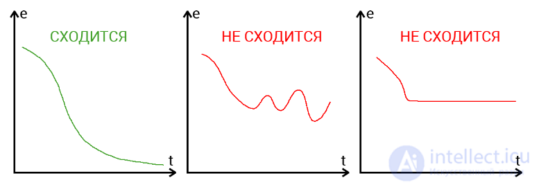
Convergence suggests whether the architecture of the National Assembly is correct and whether the hyperparameters were chosen correctly in accordance with the task. Suppose our program displays the error NA at each iteration in the log. If with each iteration the error decreases, then we are on the right track and our NA converges. If the error jumps up - down or freezes at a certain level, then the National Assembly does not converge. In 99% of cases, this is solved by changing the hyperparameters. The remaining 1% will mean that you have an error in the NA architecture. It also happens that convergence is affected by convergence.
Re-training, as the name implies, is a state of a neural network when it is oversaturated with data. This problem occurs if it takes too long to train the network on the same data. In other words, the network will begin not to learn from the data, but to memorize and “cram” them. Accordingly, when you will be already submitting new data to the input of this NA, then noise may appear in the obtained data, which will affect the accuracy of the result. For example, if we show the NA different photos of apples (only red) and say that this is an apple. Then, when the NA sees a yellow or green apple, it will not be able to determine that it is an apple, as she remembered that all apples should be red. And vice versa, when the NA sees something red and coincides in shape with an apple, for example a peach, she will say that it is an apple. This is the noise. On the graph, the noise will look like this.
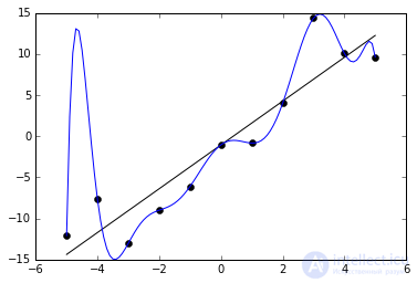
It is seen that the graph of the function varies greatly from point to point, which are the output (result) of our NA. Ideally, this graph should be less wavy and straight. To avoid retraining, it is not worth long to train the NA on the same or very similar data. Also, retraining can be caused by a large number of parameters that you apply to the input of the National Assembly or a very complex architecture. Thus, when you notice errors (noise) in the output after the training stage, then you should use one of the regularization methods, but in most cases this will not be necessary.

Comments
To leave a comment
Computational Intelligence
Terms: Computational Intelligence