Lecture
Foreword
Lab №1
Teaching with the teacher on the back-propagation error algorithm
1. Theoretical position
1.1 Artificial neuron
1.2. Activation functions
1.3. Single Layer Artificial Neural Networks
1.4. Multilayer Artificial Neural Networks
1.5. Nonlinear activation function
1.6. Network training
1.7. Pattern recognition using NA
1.8. Back Propagation Algorithm
1.9. Description of the program template and input data formats
2. Computer task
3. Variants of tasks
4. Test tasks
Literature
Artificial neural networks are an attempt to use the processes occurring in the nervous systems of living beings to develop new technological solutions.
Stanislav Osovsky
The aim of the laboratory work is to consolidate the theoretical knowledge and practical skills of working on a computer to solve artificial intelligence problems.
It is assumed that students in practical classes have already learned the basic concepts of artificial intelligence systems and have experience in the development of computer programs.
The training manual presents a cycle of one work. The first paper describes the basic methods of building and teaching a multilayer artificial neural network with a sigmoidal activation function and its training with a teacher using the back-propagation error algorithm. Chapters 1, 1.1, 1.2, 1.3, 1.4, 1.5 and 1.6 describe the general theory of NA [2]. Chapters 1.8 and 1.9 describe the error back-propagation algorithm and the class library for working with neural networks [3-6].
In laboratory studies, students compose algorithms, write programs, and carry out calculations on a computer. In the course of numerical calculations, students perform a comparative analysis of various methods of calculation for test problems. For each laboratory work a report is prepared, which contains the theory, algorithms, results of calculations, the texts of programs.
The purpose of the work: to consolidate in practice and a comparative analysis of the construction of a multi-layer, fully-connected artificial neural network of a student with a teacher using the error back-propagation algorithm.
The development of artificial neural networks is inspired by biology. That is, considering network configurations and algorithms, researchers think of them in terms of the organization of brain activity. But this analogy may end. Our knowledge of how the brain works is so limited that there would be little guidance for those who would imitate it. Therefore, network developers have to go beyond modern biological knowledge in search of structures capable of performing useful functions. In many cases, this leads to the need to abandon biological likelihood, the brain becomes just a metaphor, and networks are created that are impossible in living matter or require incredibly large assumptions about the anatomy and functioning of the brain.
The human nervous system, built from elements called neurons, has a stunning complexity. About 10 11 neurons are involved in approximately 10 15 transmission links having a meter length and more. Each neuron has many qualities that are common with other elements of the body, but its unique ability is the reception, processing and transmission of electrochemical signals along the nerve paths that form the communication system of the brain.
In fig. 1.1 shows the structure of a pair of typical biological neurons. Dendrites travel from the body of the nerve cell to other neurons, where they receive signals at junction points called synapses. The input signals received by the synapse are fed to the neuron body. Here they are summarized, and some inputs tend to excite a neuron, others - to prevent its excitation. When the total excitation in the body of a neuron exceeds a certain threshold, the neuron is excited by sending a signal along the axon to other neurons. This functional basic scheme has many complications and exceptions, however, the majority of artificial neural networks model only these simple properties.
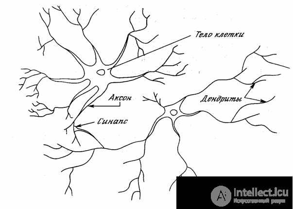
Fig. 1.1 - Biological neuron
An artificial neuron mimics in the first approximation the properties of a biological neuron. The input of an artificial neuron receives a certain set of signals, each of which is the output of another neuron. Each input is multiplied by the corresponding weight, similar to the synoptic power, and all works are summed up, determining the level of neuron activation. In fig. 1.2 presents a model that implements this idea. Although the network paradigms are very diverse, almost all of them are based on this configuration. Here, the set of input signals, denoted x 1 , x 2 , ..., x n , arrives at an artificial neuron. These input signals, collectively, denoted by the vector X , correspond to the signals arriving at the synapses of a biological neuron. Each signal is multiplied by the corresponding weight w 1 , w 2 , ... , w n , and is fed to the summing unit, denoted Σ. Each weight corresponds to the "strength" of a single biological synoptic connection. (The set of weights in the aggregate is denoted by the vector W. ) The summation block corresponding to the body of the biological element adds the weighted inputs algebraically, creating an output, which we will call NET. In vector notation, this can be compactly written as follows:
NET = XW .
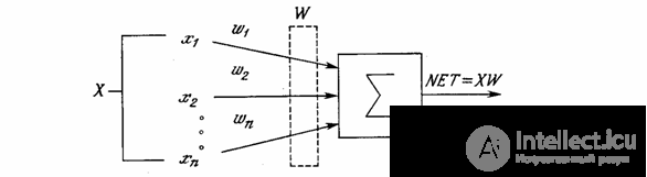
Fig. 1.2 - Artificial Neuron
The signal NET is then, as a rule, converted by the activation function F and gives the output neural signal OUT. Activation function can be a normal linear function
OUT = K (NET)
where K is a constant, threshold function
OUT = 1, if NET> T,
OUT = 0 otherwise
where T is a certain constant threshold value, or a function that more accurately simulates the nonlinear transfer characteristic of a biological neuron and represents a neural network of great potential.
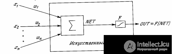
Fig. 1.3 - Artificial neuron with activation function
In fig. The 1.3 block, designated F , receives the NET signal and issues an OUT signal. If the F block narrows the range of variation of the NET value so that, for any NET values, the OUT values belong to a certain finite interval, then F is called a “compressing” function. The logistic or “sigmoidal” (S-shaped) function shown in Fig. 1 is often used as a “compressing” function. 1.4a. This function is mathematically expressed as F ( x ) = 1 / (1 + e - x ). In this way,
.
By analogy with electronic systems, the activation function can be considered a nonlinear amplification characteristic of an artificial neuron. The gain is calculated as the ratio of the increment of the OUT value to the small increment of the value NET that caused it. It is expressed by the slope of the curve at a certain level of excitation and changes from small values with large negative excitations (the curve is almost horizontal) to a maximum value with zero excitation and decreases again when the excitation becomes large positive. Grossberg (1973) discovered that a similar nonlinear characteristic solves the noise saturation dilemma he poses. How can the same network handle both weak and strong signals? Weak signals need large network amplification to give usable output. However, amplifier stages with high gains can lead to saturation of the output with amplifier noise (random fluctuations) that are present in any physically implemented network. Strong input signals in turn will also lead to saturation of the amplifier stages, eliminating the possibility of useful output. The central region of the logistic function, which has a large gain, solves the problem of processing weak signals, while the regions with a falling gain at the positive and negative ends are suitable for large excitations. Thus, the neuron functions with high gain in a wide range of input signal level.
. 
Fig. 1.4a - Sigmoidal logistic function
Another widely used activation function is the hyperbolic tangent. It is similar in shape to the logistic function and is often used by biologists as a mathematical model of nerve cell activation. As the activation function of an artificial neural network, it is written as follows:
OUT = th (x).
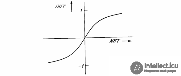
Fig. 1.4b - Hyperbolic tangent function
Like the logistic function, the hyperbolic tangent is an S-shaped function, but it is symmetric about the origin, and at the point NET = 0 the value of the output signal OUT is zero (see Fig. 1.4b). Unlike the logistic function, the hyperbolic tangent takes on the values of different signs, which turns out to be beneficial for a number of networks.
The considered simple model of an artificial neuron ignores many properties of its biological twin. For example, it does not take into account the time delays that affect the dynamics of the system. The input signals immediately generate the output signal. And, more importantly, it does not take into account the effects of the frequency modulation function or the synchronizing function of a biological neuron, which some researchers consider decisive.
Despite these limitations, networks built from these neurons exhibit properties that strongly resemble a biological system. Only time and research will be able to answer the question whether such coincidences are random or because the model correctly captures the most important features of a biological neuron.
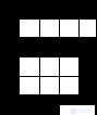
Although one neuron is capable of performing the simplest recognition procedures, the power of neural computing results from the connections of neurons in networks. The simplest network consists of a group of neurons forming a layer, as shown in the right-hand side of Fig. 1.5. Note that the circle tops on the left serve only for the distribution of input signals. They do not perform any calculations, and therefore will not be considered a layer. For this reason, they are indicated by circles to distinguish them from the computing neurons, indicated by squares. Each element of the set of inputs X is connected with a separate weight to each artificial neuron. And each neuron provides a weighted sum of network inputs. In artificial and biological networks, many compounds may be missing; all compounds are shown for generality purposes. Connections between the outputs and the inputs of the elements in the layer may also take place.
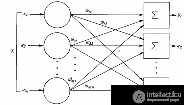
Fig. 1.5 - Single Layer Neural Network
It is convenient to consider the weight of the elements of the matrix W. The matrix has m rows and n columns, where m is the number of inputs, and n is the number of neurons. For example, w 2,3 is the weight connecting the third input to the second neuron. Thus, the calculation of the output vector N , whose components are the outputs OUT of neurons, is reduced to the matrix multiplication N = XW , where N and X are row vectors.
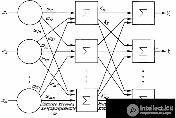
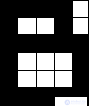
Fig. 1.6 - Dual Layer Neural Network
Larger and more complex neural networks have, as a rule, large computational capabilities. Although networks of all configurations that can be imagined are created, the layered organization of neurons copies the layered structures of certain parts of the brain. It turned out that such multi-layer networks have greater capabilities than single-layer networks, and in recent years algorithms have been developed for their training.
Multilayer networks can be formed in cascades of layers. The output of one layer is the entrance to the next layer. A similar network is shown in Fig. 1.6 and again depicted with all connections.
Multilayer networks cannot lead to an increase in computational power compared to a single-layer network only if the activation function between the layers is nonlinear. The calculation of the layer output consists in multiplying the input vector by the first weight matrix followed by multiplication (if there is no nonlinear activation function) of the resulting vector by the second weight matrix.
( XW 1 ) W 2
Since matrix multiplication is associative,
X ( W 1 W 2 ).
This shows that a two-layer linear network is equivalent to one layer with a weight matrix equal to the product of two weight matrices. Consequently, any multi-layered linear network can be replaced by an equivalent single-layer network. In ch. 2 shows that single-layer networks are very limited in their computing capabilities. Thus, in order to expand the capabilities of networks compared to a single-layer network, a non-linear activation function is necessary.
The network is trained in order for some set of inputs to give the desired (or, at least, consistent with it) set of outputs. Each such input (or output) set is considered as a vector. Training is carried out by sequential presentation of input vectors with simultaneous adjustment of the weights in accordance with a specific procedure. In the process of learning, the weights of the network gradually become such that each input vector produces an output vector.
There are learning algorithms with and without a teacher. Teaching with a teacher assumes that for each input vector there is a target vector representing the required output. Together they are called a learning pair. Typically, the network is trained on a number of such training pairs. The output vector is presented, the network output is calculated and compared with the corresponding target vector, the difference (error) is fed into the network using feedback, and the weights are changed in accordance with an algorithm that tends to minimize the error. The training set vectors are presented sequentially, errors are calculated and weights are adjusted for each vector until the error across the entire training array reaches an acceptably low level.
Despite numerous applied advances, teaching with the teacher was criticized for its biological improbability. It is difficult to imagine a learning mechanism in the brain that would compare the desired and actual output values, performing a correction using feedback. If we allow a similar mechanism in the brain, then where do the desired outputs come from? Teaching without a teacher is a much more plausible model of learning in a biological system. Developed by Kohonen and many others, it does not need a target vector for exits and, therefore, does not require comparison with predetermined ideal answers. The training set consists only of input vectors. The learning algorithm adjusts the weights of the network so that consistent output vectors are obtained, that is, the presentation of sufficiently close input vectors gives the same outputs. The learning process, therefore, highlights the statistical properties of the training set and groups similar vectors into classes. The presentation of a vector from a given class to an input will give a certain output vector, but before learning it is impossible to predict what output will be made by this class of input vectors. Consequently, the outputs of such a network should be transformed into some understandable form, due to the learning process. This is not a serious problem. It is usually not difficult to identify the connection between the input and the output established by the network.
NA used to solved a wide range of tasks. Application areas NA:
Consider an example of pattern recognition using NA. As a mathematical representation of the image, we will understand a matrix of numbers in which elements can take only two values: -0.5 and 0.5. Where -0.5 will conditionally correspond to the black pixel of the image, and 0.5 to white. For example, for images consisting of the letters “A”, “B” and “C”, the matrix and the graphic black-and-white image are shown in Table 1.
Image name | "BUT" | “B” | "AT" |
Black and white image |
|
|
|
Matrix 5x6 | |||
The 5x6 matrix in which, for clarity, -0.5 is replaced by “.” And 0.5 by “X”. | ..X .. .XX X ... X XXXXX X ... X X ... X | XXXXX X .... XXXXX X ... X X ... X XXXXX | XXXX. H.H. XXXXX X ... X X ... X XXXXX |
Table 1 - Representation of images by matrix of coefficients
The input data of the NA is a vector, so our source data must be converted to a vector view. We can represent the nxm matrix in the form of a vector of length n * m, by writing the coefficients of the matrix to a vector line by line. For a 5x6 matrix, the corresponding vector will contain 30 elements.
Matrix | ..X .. .XX X ... X XXXXX X ... X X ... X |
vector | ..X ... xxx X ... X XXXXX X ... X X ... X |
Таблица 2 – Представление матрицы в виде вектора
Выходными данными НС являются тоже вектор. Этот вектор мы должны интерпретировать в терминах решаемой задачи. Зададим размерность выходного вектора сети равным количеству распознаваемых образов. Для нашей задачи размерность равна – 3. Пусть образам “А”, “Б” и “В” соответствуют классы 1, 2 и 3. Тогда выходной вектор, соответствующий классу n будет иметь значение 0.5 в n-ой позиции и -0.5 в остальных. Пример приведен в таблице 3.
Название класса | “А” | “Б” | “В” |
Номер класса | one | 2 | 3 |
Выходной вектор | Х.. | .Х. | ..Х |
Таблица 3 – соответствие выходных векторов классам.
The pattern of use of the INS is shown in Figure 1.7. The input to the INS is the symbol that needs to be recognized. INS calculates its coefficients and gives the result. Only those characters that were taught to her or those close to her (distorted or noisy) can recognize the ANN.
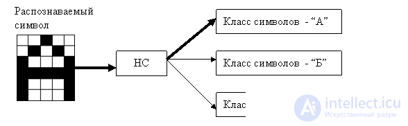
Fig. 1.7 - scheme of use of NA
Среди различных структур нейронных сетей (НС) одной из наиболее известных является многослойная структура, в которой каждый нейрон произвольного слоя связан со всеми аксонами нейронов предыдущего слоя или, в случае первого слоя, со всеми входами НС. Такие НС называются полносвязными. Когда в сети только один слой, алгоритм ее обучения с учителем довольно очевиден, так как правильные выходные состояния нейронов единственного слоя заведомо известны, и подстройка синаптических связей идет в направлении, минимизирующем ошибку на выходе сети. По этому принципу строится, например, алгоритм обучения однослойного персептрона. В многослойных же сетях оптимальные выходные значения нейронов всех слоев, кроме последнего, как правило, не известны, и двух или более слойный персептрон уже невозможно обучить, руководствуясь только величинами ошибок на выходах НС. Один из вариантов решения этой проблемы – разработка наборов выходных сигналов, соответствующих входным, для каждого слоя НС, что, конечно, является очень трудоемкой операцией и не всегда осуществимо. Второй вариант – динамическая подстройка весовых коэффициентов синапсов, в ходе которой выбираются, как правило, наиболее слабые связи и изменяются на малую величину в ту или иную сторону, а сохраняются только те изменения, которые повлекли уменьшение ошибки на выходе всей сети. Очевидно, что данный метод "тыка", несмотря на свою кажущуюся простоту, требует громоздких рутинных вычислений. И, наконец, третий, более приемлемый вариант – распространение сигналов ошибки от выходов НС к ее входам, в направлении, обратном прямому распространению сигналов в обычном режиме работы. Этот алгоритм обучения НС получил название процедуры обратного распространения. Именно он будет рассмотрен в дальнейшем.
Согласно методу наименьших квадратов, минимизируемой целевой функцией ошибки НС является величина:
 (one)
(one)
где – реальное выходное состояние нейрона j выходного слоя N нейронной сети при подаче на ее входы p-го образа; d jp – идеальное (желаемое) выходное состояние этого нейрона.
Суммирование ведется по всем нейронам выходного слоя и по всем обрабатываемым сетью образам. Минимизация ведется методом градиентного спуска, что означает подстройку весовых коэффициентов следующим образом:
 (2)
(2)
Здесь w ij – весовой коэффициент синаптической связи, соединяющей i-ый нейрон слоя n-1 с j-ым нейроном слоя n, h – коэффициент скорости обучения, 0<h <1.
 (3)
(3)
Здесь под y j , как и раньше, подразумевается выход нейрона j, а под s j – взвешенная сумма его входных сигналов, то есть аргумент активационной функции. Так как множитель dy j / ds j является производной этой функции по ее аргументу, из этого следует, что производная активационной функция должна быть определена на всей оси абсцисс. В связи с этим функция единичного скачка и прочие активационные функции с неоднородностями не подходят для рассматриваемых НС. В них применяются такие гладкие функции, как гиперболический тангенс или классический сигмоид с экспонентой. В случае гиперболического тангенса
 (four)
Третий множитель ¶ s j /¶ w ij , очевидно, равен выходу нейрона предыдущего слоя y i (n-1) .
Что касается первого множителя в (3), он легко раскладывается следующим образом[2]:
 (five)
Здесь суммирование по k выполняется среди нейронов слоя n+1.
Введя новую переменную
 (6)
(6)
мы получим рекурсивную формулу для расчетов величин d j (n) слоя n из величин d k (n+1) более старшего слоя n+1.
 (7)
(7)
Для выходного же слоя
 (eight)
Теперь мы можем записать (2) в раскрытом виде:
 (9)
(9)
Иногда для придания процессу коррекции весов некоторой инерционности, сглаживающей резкие скачки при перемещении по поверхности целевой функции, (9) дополняется значением изменения веса на предыдущей итерации
 (ten)
(ten)
где m – коэффициент инерционности, t – номер текущей итерации.
Таким образом, полный алгоритм обучения НС с помощью процедуры обратного распространения строится так:
1. Подать на входы сети один из возможных образов и в режиме обычного функционирования НС, когда сигналы распространяются от входов к выходам, рассчитать значения последних. Напомним, что
 (eleven)
где M – число нейронов в слое n-1 с учетом нейрона с постоянным выходным состоянием +1, задающего смещение; y i (n-1) =x ij (n) – i-ый вход нейрона j слоя n.
y j (n) = f(s j (n) ) , где f() – сигмоид (12)
y q (0) =I q , (13)
где I q – q-ая компонента вектора входного образа.
2. Рассчитать d (N) для выходного слоя по формуле (8).
Рассчитать по формуле (9) или (10) изменения весов D w (N) слоя N.
3. Рассчитать по формулам (7) и (9) (или (7) и (10)) соответственно d (n) и D w (n) для всех остальных слоев, n=N-1,...1.
4. Скорректировать все веса в НС
 (14)
(14)
5. Если ошибка сети существенна, перейти на шаг 1. В противном случае – конец.
Сети на шаге 1 попеременно в случайном порядке предъявляются все тренировочные образы, чтобы сеть, образно говоря, не забывала одни по мере запоминания других. Алгоритм иллюстрируется рисунком 1.
Из выражения (9) следует, что когда выходное значение y i (n-1) стремится к нулю, эффективность обучения заметно снижается. При двоичных входных векторах в среднем половина весовых коэффициентов не будет корректироваться[3], поэтому область возможных значений выходов нейронов [0,1] желательно сдвинуть в пределы [-0.5,+0.5], что достигается простыми модификациями логистических функций. Например, сигмоид с экспонентой преобразуется к виду
(15)
Как видно из формул, описывающих алгоритм функционирования и обучения НС, весь этот процесс может быть записан и затем запрограммирован в терминах и с применением операций матричной алгебры. Судя по всему, такой подход обеспечит более быструю и компактную реализацию НС, нежели ее воплощение на базе концепций объектно-ориентированного (ОО) программирования. Однако в последнее время преобладает именно ОО подход, причем зачастую разрабатываются специальные ОО языки для программирования НС, хотя, с моей точки зрения, универсальные ОО языки, например C++ и Pascal, были созданы как раз для того, чтобы исключить необходимость разработки каких-либо других ОО языков, в какой бы области их не собирались применять.
И все же программирование НС с применением ОО подхода имеет свои плюсы. Во-первых, оно позволяет создать гибкую, легко перестраиваемую иерархию моделей НС. Во-вторых, такая реализация наиболее прозрачна для программиста, и позволяет конструировать НС даже непрограммистам. В-третьих, уровень абстрактности программирования, присущий ОО языкам, в будущем будет, по-видимому, расти, и реализация НС с ОО подходом позволит расширить их возможности. Исходя из вышеизложенных соображений, приведенная в листингах библиотека классов и программ, реализующая полносвязные НС с обучением по алгоритму обратного распространения, использует ОО подход. Вот основные моменты, требующие пояснений.
Прежде всего необходимо отметить, что библиотека была составлена и использовалась в целях распознавания изображений, однако применима и в других приложениях. В файле neuro.h в приведены описания двух базовых и пяти производных (рабочих) классов: Neuron, SomeNet и NeuronFF, NeuronBP, LayerFF, LayerBP, NetBP, а также описания нескольких общих функций вспомогательного назначения, содержащихся в файле subfun.cpp. Методы пяти вышеупомянутых рабочих классов внесены в файлы neuro_ff.cpp и neuro_bp.cpp, представленные в приложении. Такое, на первый взгляд искусственное, разбиение объясняется тем, что классы с суффиксом _ff, описывающие прямопоточные нейронные сети (feedforward), входят в состав не только сетей с обратным распространением – _bp (backpropagation), но и других, например таких, как с обучением без учителя, которые будут рассмотрены в дальнейшем.
To the detriment of the principles of OO programming, the six main parameters characterizing the operation of the network are brought to the global level, which facilitates operations with them. The SigmoidType parameter defines the type of activation function. The NeuronFF :: Sigmoid method lists some of its values, the macros of which are made in the header file. HARDLIMIT and THRESHOLD items are given for generality, but cannot be used in the back-propagation algorithm, since the corresponding activation functions have derivatives with special points. This is reflected in the method of calculating the derivative NeuronFF :: D_Sigmoid, from which these two cases are excluded. The variable SigmoidAlfa sets the slope of a sigmoid ORIGINAL from (15). MiuParm and NiuParm are, respectively, the values of the parameters m and h from formula (10). The Limit value is used in the IsConverged methods to determine when the network learns or becomes paralyzed. In these cases, the changes in the weights become smaller than the small Limit value. The dSigma parameter emulates the density of noise added to the images during NA learning. This allows you to generate a virtually unlimited number of noisy images from a finite set of "clean" input images. The fact is that in order to find the optimal values of the weighting factors, the number of degrees of freedom NA — N w must be much less than the number of restrictions imposed — N y × N p , where N p is the number of images presented by the National Assembly during training. In fact, the dSigma parameter is equal to the number of inputs that will be inverted in the case of a binary image. If dSigma = 0, no interference is introduced.
Randomize methods allow you to set weights to random values in the range [-range, + range] before starting the training. Propagate methods perform calculations using formulas (11) and (12). The NetBP :: CalculateError method, based on the array of valid (desired) output values of the NA, transmitted as an argument, calculates d values. The NetBP :: Learn method calculates changes in weights using the formula (10), the Update methods update weighting factors. The NetBP :: Cycle method combines all the procedures of a single learning cycle, including setting the input signals NetBP :: SetNetInputs. The various methods PrintXXX and LayerBP :: Show allow you to control the flow of processes in the NA, but their implementation is not critical, and simple procedures from the given library can be rewritten, if desired, for example, for the graphic mode. This is also justified by the fact that in alphanumeric mode it is no longer possible to fit on the screen information about a relatively large NA.
Networks can be constructed using NetBP (unsigned), after which they need to be filled with previously constructed layers using the NetBP :: SetLayer method, or using NetBP (unsigned, unsigned, ...). In the latter case, layer constructors are called automatically. To establish the synaptic connections between the layers, the NetBP :: FullConnect method is called.
After the network has been trained, its current state can be written to a file (NetBP :: SaveToFile method), and then restored using the NetBP :: LoadFromFile method, which is applicable only to the network just constructed using NetBP (void).
For input to the network of input images, and at the training stage - and for setting weekends, three methods are written: SomeNet :: OpenPatternFile, SomeNet :: ClosePatternFile and NetBP :: LoadNextPattern. If the image files have an arbitrary extension, the input and output vectors are written alternatingly: a line with an input vector, a line with a corresponding output vector, and so on. Each vector is a sequence of real numbers in the range [-0.5, + 0.5], separated by an arbitrary number of spaces. If the file has the IMG extension, the input vector is represented as a matrix of characters of dy * dx size (dx and dy values must be set in advance using LayerFF :: SetShowDim for the zero layer), with the 'x' character corresponding to level 0.5, and the dot to level -0.5, that is, IMG files, at least in the given version of the library, are binary. When the network is operating normally, and not learning, the lines with the output vectors may be empty. The SomeNet :: SetLearnCycle method sets the number of passes through the image file, which, combined with the addition of noise, allows you to get a set of several tens or even hundreds of thousands of different images.
Now let us touch on the issue of the capacity of the NA, that is, the number of images shown at its inputs, which it can learn to recognize. For networks with more than two layers, it remains open. As shown in [4], for an NS with two layers, that is, an output and one hidden layer, the deterministic capacity of the C d network is estimated as follows:
N w / N y <C d <N w / N y × log (N w / N y ) (16)
where N w is the number of adjustable weights, N y is the number of neurons in the output layer.
It should be noted that this expression was obtained subject to some restrictions. First, the number of inputs of N x and neurons in the hidden layer N h must satisfy the inequality N x + N h > N y . Secondly, N w / N y > 1000. However, the above assessment was carried out for networks with activation functions of neurons in the form of a threshold, and the capacity of networks with smooth activation functions, for example (15), is usually greater. In addition, the adjective “deterministic” appearing in the capacity name means that the resulting capacity estimate is absolutely suitable for all possible input images that can be represented by N x inputs. In fact, the distribution of input images, as a rule, has some regularity, which allows the NA to carry out a generalization and, thus, increase the actual capacity. Since the distribution of images, in general, is not known in advance, we can only talk about such capacity presumably, but usually it is twice as large as the deterministic capacity.
In continuation of the discussion on the capacity of the National Assembly, it is logical to raise the question of the required capacity of the output network layer that performs the final classification of the images. The fact is that for the separation of a set of input images, for example, in two classes, only one output is sufficient. In addition, each logic level - "1" and "0" - will denote a separate class. On the two outputs, it is already possible to encode 4 classes and so on. However, the results of the network, organized in this way, we can say - "to the eyeballs" - are not very reliable. To increase the classification accuracy, it is desirable to introduce redundancy by allocating each class a single neuron in the output layer or, even better, several, each of which is trained to determine the image belonging to the class with its degree of confidence, for example: high, medium and low. Such NAs allow classification of input images combined into fuzzy (fuzzy or intersecting) sets. This property brings similar NA to the conditions of real life.
The NA has several bottlenecks. Firstly, in the process of learning, a situation may arise when large positive or negative values of the weighting factors shift the working point on the sigmoids of many neurons to the saturation region. Small values of the derivative of the logistic function will, in accordance with (7) and (8), stop learning, which paralyzes the NA. Secondly, the use of the gradient descent method does not guarantee that a global minimum, rather than a local minimum, of the objective function will be found. This problem is connected with one more, namely with the choice of the magnitude of the learning rate. Proof of convergence of learning in the process of backward propagation is based on derivatives, that is, the increments of weights and, therefore, the learning rate must be infinitely small, but in this case learning will be unacceptably slow. On the other hand, too large corrections of weights can lead to a constant instability of the learning process. Therefore, h is usually chosen as a number less than 1, but not very small, for example, 0.1, and, generally speaking, it can gradually decrease in the learning process. In addition, to exclude random hits to local minima, sometimes, after the values of the weighting coefficients stabilize, h is briefly greatly increased to begin the gradient descent from the new point. If repeating this procedure several times will bring the algorithm to the same state of the NA, you can more or less confidently say that a global maximum has been found, and not some other.
There is another method for eliminating local minima, as well as paralysis of the NA, which consists in the use of stochastic NA, but it is better to talk about them separately.
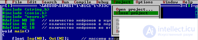
2.1 Make a copy of the neuro folder and rename it for example “labrab”. Leave the neuro folder untouched for the sample, in case of difficulties with the program from there you can always get a working code. Open Borland C ++ 3.1 and make the labrab folder the working directory. To do this, select the menu item File-> Change dir

Select the labrab directory on your computer.
Select in the menu item Project->
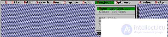
Open project teacher.prj
Run the program - CTRL-F9
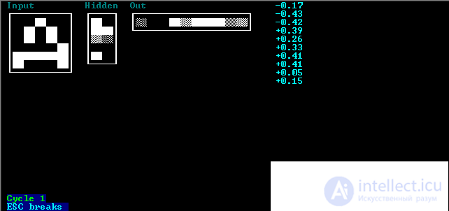
The program waits for a command from the user. If you press ESC, the program ends. If you press ENTER, the program will perform one training cycle.

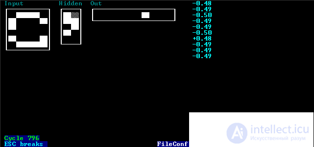
The results of one training cycle will be displayed on the screen. The input vector (network zero layer) is called “Input”, the first network layer (hidden) is “Hidden” and the second network layer (output) is “Out”. For clarity, the input vector is not displayed as a vector but as a 5x6 matrix, the intermediate layer is a 2x5 matrix, and the output layer is a 10x1 matrix. The screen displays the value of neuronal axons in all layers of the 0-2 network. In the zero layer there are 30 neurons, in the intermediate 10 and output 10. The value of each axon of the neuron lies in the range [-0.5; 0.5]. Black color corresponds to -0.5, and white 0.5. Also, in the upper right corner, the axon values of the neurons of the output layer are displayed in a numerical format. If you press any key, the learning process will pass automatically and stop when the specified accuracy is reached.
After stopping the training, the program will offer to save the weights of the NA to a file. If you enter an empty string, the saving is performed, will not. Save the weights of the NA in the file wesa.txt. View this file, such as notepad. Now let's start using a trained NS. Close the project. (Note: if the network parameters are not matched successfully, then the learning process will not end when. This may be due to the small number of neurons in the hidden layer. This can be due to large learning factors and noise).
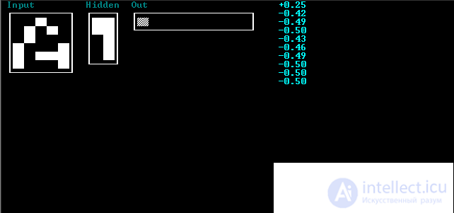
Open the project use.prj. Run the program. Displaying results is similar to the description of the teacher program. The input vector is the tested vector. The values of the intermediate layer are not interpreted as. The index of the maximum element in the output array corresponds to the class number to which the NA assigned the recognizable character. When you press any key, the next vector from the file will be recognized. The process ends when the data runs out.
2.1 Using the training program (teacher) given in the “test tasks” section, build a two-layer neural network and train it to recognize graphic images from an individual task.
2.2 Save network weights to file. Then load the weights from the file into the program and test the network with examples not provided to it during training. Use the tutorial (use).
2.3 Determine the maximum number of neurons in the intermediate layer, in which the learning process is not when it does not end.
2.4 Enter noise in the training set and repeat the training, save the weights to a file. Compare the trainee recognition results with and without noise.
2.5 Prepare a report containing the following items:
3.1 digits 0..9 6x6 matrix
3.2 ten letters of the Latin alphabet 6x7 matrix
3.3 ten letters of the Russian alphabet 7x6 matrix
3.4 five road signs 8x8 matrix
4.1. Text of the main curriculum (teacher.cpp)
#include <string.h>
#include <conio.h>
#include "neuro.h"
void main ()
{
int N0 = 30; // number of neurons in the zero layer
int N1 = 10; // number of neurons in the first layer
int N2 = 10; // number of neurons in the second layer
NetBP N (3, N0, N1, N2); // constructor for creating a network of three layers
// the zero layer is dummy and does not participate in the calculations
// it is needed to store the input data vector
// so the network will disappear two-layer
float * Inp, * Out; // arrays of network input and output
Inp = new float [N0]; // array of network input data
Out = new float [N2]; // array of network output
unsigned count; // number of network learning cycles
unsigned char buf [256]; // buffer for text processing
int i; // stores the key code
ClearScreen (); // clear the screen
N.FullConnect (); // linking network layers to each other
N.GetLayer (0) -> SetName ("Input"); // set the name of the layer
N.GetLayer (0) -> SetShowDim (1,1,5,6); // assignment of coordinates
// and form output layer on the screen
N.GetLayer (1) -> SetName ("Hidden"); // set the name of the layer
N.GetLayer (1) -> SetShowDim (15,1,2,5); // task of coordinates
// and form output layer on the screen
N.GetLayer (2) -> SetName ("Out"); // set the name of the layer
N.GetLayer (2) -> SetShowDim (23,1,10,1); // task of coordinates
// and form output layer on the screen
N.SaveToFileConfigShow ("config.txt"); // save parameters to file
// display layers on screen
SetSigmoidType (HYPERTAN); // setting the type of activation function
// HYPERTAN - hyperbolic tangent (recommended)
// ORIGINAL - sigmoid
SetNiuParm (0.1); // network training coefficient lies in the interval 0..1
// Recommended to use 0.1
// with a small value, the training will take a very long time
// when large - old network skills will be completely replaced by new ones
// and the learning process is not when not to end
SetLimit (0.001); // Limit value is used in IsConverged methods.
// to determine when the network learns or falls into
// paralysis. In these cases, changes in weights become less
// low limit (0.001 is recommended)
SetDSigma (1); // DSigma parameter emulates noise density
// added to the images during training NA.
// Actually, the DSigma parameter is equal to the number of inputs that will be
// inverted in the case of a binary image.
// If DSigma = 0, no interference is introduced. (recommended 1, 2)
N.Randomize (1); // Randomize methods allow before starting
// learning to set weights to random
// values in the range [-range + range]. (recommended 1)
N.SetLearnCycle (64000U); // SomeNet :: SetLearnCycle method sets
// number of passes through the image file, which in combination with
// adding noise allows you to get a set of several
// tens and even hundreds of thousands of different images.
// (64000U recommended)
N.OpenPatternFile ("teacher.img"); // file name with the training set
// If image files have an arbitrary extension?
// then the input and output vectors are written alternatingly,
// string with input vector, string with corresponding to it
// output vector, etc. Each vector is a sequence
// real numbers in the range [-0.5, + 0.5], separated
// arbitrary number of spaces. If the file has an img extension,
// input vector is represented as a matrix of characters
// size dy * dx (dx and dy values must be in advance
// set using LayerFF :: SetShowDim for the zero layer),
// with the 'x' character or any other character except
// character point corresponds to level 0.5,
// and the dot is -0.5 level, i.e. IMG files,
// at least in the given library version,
// binary. When the network is working normally,
// rather than learning, the lines with the output vectors may be empty.
i = 13; // Enter key code - 13
for (count = 0 ;; count ++) // main learning cycle
{
if (N.LoadNextPattern (Inp, Out)) break; // load a pair from the file
// input and output vector
N.Cycle (Inp, Out); // teach the network with the current example.
N.GetLayer (0) -> Show (); // display on the screen of the zero layer
N.GetLayer (1) -> Show (); // display the first layer on the screen
N.GetLayer (2) -> Show (); // display the second layer
N.GetLayer (2) -> PrintAxons (47.0); // display of coefficients
// second layer
sprintf (buf, "Cycle% u", count); // form a string with information
// about the number of cycles
out_str (1.23, buf, 10 | (1 << 4)); // display the number of cycles on the screen
out_str (1.24, "ESC breaks", 11 | (1 << 4)); // display a hint
if (kbhit () || i == 13) i = getch (); // if the key is pressed or earlier
// Enter was pressed then read the code of the pressed key
if (i == 27) break; // if ESC is pressed, then completion of training and exit
if (i == 's' || i == 'S') goto save; // if the 's' key is pressed then
// switch to file saving
if (count && N.IsConverged ()) // if the network is trained then saving
{
save:
out_str (40,24, "FileConf:", 15 | (1 << 4)); // display the message
gotoxy (50.25); // position the cursor
gets (buf); // enter the file name to save the network weights
if (strlen (buf)) N. SaveToFile (buf); // if the file name is not empty
// then save the weight in the file
break; // completion of the learning cycle
}
}
N.ClosePatternFile (); // close the file with the training set
delete [] Inp; // array of network input data
delete [] Out; // array of network output
}
4.2. Text of the input file with the training sample (teacher.img)
..x ..
.xx
.xx
x ... x
xxxxx
x ... x
A .........
x ... x
xx.xx
xx.xx
xxx
xxx
x ... x
.M ........
x ... x
x ... x
xxxxx
x ... x
x ... x
x ... x
..H .......
x ... x
x..xx
xxx
xxx
xx..x
x ... x
... N ......
x..xx
xx.
xx ...
xx.
x..x.
x ... x
.... K .....
... x.
..xx
.x..x
x ... x
x ... x
x ... x
..... L ....
.xxx.
x ... x
x ....
x ....
x ... x
.xxx
...... C ...
xxxxx
..x ..
..x ..
..x ..
..x ..
..x ..
....... T ..
xxxxx
x ... x
x ... x
x ... x
x ... x
x ... x
........ P.
xxxx.
x ... x
xxxx
x ... x
x ... x
xxxx.
......... B
4.1. Text of the main test program (use.cpp)
#include <string.h>
#include <conio.h>
#include "neuro.h"
main ()
{
NetBP N;
if (N.LoadFromFile ("wesa.txt")) {
out_str (1.24, "I can not open the scale file.", 11 | (1 << 4));
getch ();
return 1;}; // build a network based on
// file of network weights obtained as a result of training
if (N.FullConnect ()) {
out_str(1,24,"Не соответствие файла весов и параметров сети.",11 | (1<<4));
getch();
return 1;}; // связывание слоев сети друг с другом
ClearScreen(); // очистка экрана
float *Inp, *Out;// массивы входных и выходных данных сети
Inp = new float [N.GetLayer(0)->GetRang()]; // массив входных данных сети
Out = new float [N.GetLayer(N.GetRang()-1)->GetRang()]; // массив выходных данных сети
switch (N.LoadFromFileConfigShow("config.txt")){
case 1:
out_str(1,24,"Не могу открыть файл конфигурации отображения на экран.",11 | (1<<4));
getch();
return 1;
case 2:
out_str(1,24,"Не соответствие файла конфигурации и количества слоев сети.",11 | (1<<4));
getch();
return 1;
}; // открытие файла конфигурации отображения на экран
// этот файл формируется при обучении сети и в нем хранятся
// имена слоев сети, положение на экране и формат вывода.
SetSigmoidType(HYPERTAN);// задание вида активационной функции
// HYPERTAN - гиперболический тангенс (рекомедуется)
// ORIGINAL - сигмоид
if(N.OpenPatternFile("use.img")) {
out_str(1,24,"Не могу открыть файл с тестируемой выборкой.",11 | (1<<4));
getch();
return 1;};// имя файла с тестируемой выборкой
// Если у файлов образов произвольное расширение?
// то входные и выходные вектора записываются чередуясь,
// строка с входным вектором, строка с соответствующим ему
// выходным вектором и т.д. Каждый вектор есть последовательность
// действительных чисел в диапазоне [-0.5,+0.5], разделенных
// произвольным числом пробелов. Если файл имеет расширение IMG,
// входной вектор представляется в виде матрицы символов
// размером dy*dx (величины dx и dy должны быть заблаговременно
// установлены с помощью LayerFF::SetShowDim для нулевого слоя),
// причем символ 'x' или любой другой символ кроме
// символа точка соответствует уровню 0.5,
// а точка - уровню -0.5, то есть файлы IMG,
// по крайней мере - в приведенной версии библиотеки,
// бинарны. Когда сеть работает в нормальном режиме,
// а не обучается, строки с выходными векторами могут быть пустыми.
int i=13; // код клавиши Enter - 13
for(;;)// основной цикл тестирования
{
if(N.LoadNextPattern(Inp,Out)) break;// загружаем из файла пару
// входного и выходного вектора в данной программе
// выходной вектор не нужен
// когда образци кончатся то завершаем цикл тестирования
N.SetNetInputs(Inp); // заносим вектор входных данных в сеть
N.Propagate(); // прощитываем значение сети
N.GetLayer(0)->Show(); // вывод на экран нулевого слоя
N.GetLayer(1)->Show(); // вывод на экран первого слоя
N.GetLayer(2)->Show(); // вывод на экран второго слоя
N.GetLayer(2)->PrintAxons(47,0); // вывод на экран коэфициентов
// второго слоя
if(kbhit() || i==13) i=getch(); // если нажата клавиша или раньше
// был нажат Enter тогда считать код нажатой клавиши
if(i==27) break;// если нажат ESC то завершение обучения и выход
}
N.ClosePatternFile();// закрытие файла с тестирующей выборкой
delete [] Inp; // массив входных данных сети
delete [] Out; // массив выходных данных сети
return 0;
}
4.4 Текст входного файла с тестируемой выборкой (use.img)
..x..
.xx
.x...
x...x
x.xxx
x...x
A.........
x...x
xx.xx
xx.xx
..xx
xxx
x....
.M........
x...x
x....
xx.xx
x...x
x...x
x...x
..H.......
x...x
x..x.
xxx
..xx
xx..x
x...x
...N......
...xx
xx.
x....
xx.
x..x.
x...x
....K.....
...x.
..xx
.x…
x...x
....x
x...x
.....L....
.xx..
x...x
x....
.....
x...x
.xxx
......C...
x.xxx
..x..
..x..
..x..
…..
..x..
.......T..
x.xxx
x...x
x...x
x...x
x....
x...x
........P.
xxxx.
....x
xxxx
x..xx
x....
xxxx.
.........B
1. Осовский С. Нейронные сети для обработки информации / Пер. с польского И.Д. Рудинского. – М.: Финансы и статистика, 2002. – 344 с.: ил.
2. Уоссермен Ф. Нейрокомпьютерная техника: теория и практика. — М.: Мир, 1992.
3. С. Короткий Нейронные сети: основные положения - Электронная публикация.
4. С. Короткий Нейронные сети: алгоритм обратного распространения - Электронная публикация.
5. С. Короткий Нейронные сети: Нейронные сети: обучение без учителя - Электронная публикация.
6. С. Короткий Нейронные сети Хопфилда и Хэмминга - Электронная публикация.


Comments
To leave a comment
Models and research methods
Terms: Models and research methods