Introduction
I will immediately inform you that the post has nothing to do with perceptrons, Hopfield networks or any other artificial neural networks. We will simulate the work of a “real”, “living”, biological neural network in which the processes of generation and propagation of nerve impulses occur. In English-language literature, such networks are called spiking neural networks due to their difference from artificial neural networks, while Russian-language literature does not have a well-established name, someone calls them simply neural networks, someone impulsive neural networks, someone spike, and some it is generally neural networks.
Probably the majority of readers have heard about the Blue Brain and Human Brain projects sponsored by the European Union, for the latest project the EU government issued about a billion euros, which indicates a great interest in this area. Both projects are closely related and intersect with each other, even the head of them is common, Henry Markram, which can create some confusion about how they differ from each other. In short, the ultimate goal of both projects is to develop a model of the whole brain (all 86 billion neurons) and its subsequent modeling on a supercomputer. The Blue Brain Project is the computational part, and the Human Brain is more of a fundamental part, where they work on collecting scientific data on the principles of the brain and creating a single model. In order to touch this science and try to do something similar ourselves, albeit on a much smaller scale, this article was written.
But they did not address issues of computational neuroscience, or in another way computational neuroscience, which includes computer modeling of the electrical activity of neurons. Therefore, I decided to fill this gap.
Some biology
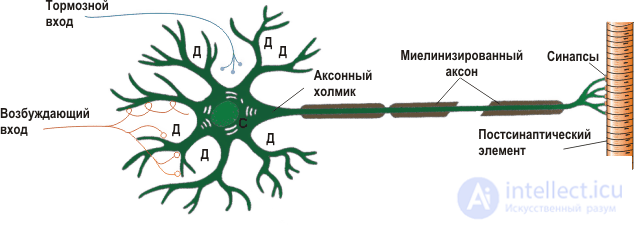 Fig. 1 - Schematic representation of the structure of the neuron.
 Before we start modeling, we need to familiarize ourselves with some of the basics of neurobiology. A typical neuron consists of 3 parts: the body (soma), dendrites and axon. Dendrites receive a signal from other neurons (this is the input of the neuron), and the axon transmits signals from the body of the neuron to other neurons (output). The site of contact of the axon of one neuron and the dendrite of another neuron is called a synapse. The signal received from the dendrites is summed up in the body, and if it exceeds a certain threshold, a nerve impulse is generated or, in another way, a spike. The cell body is surrounded by a lipid membrane, which is a good insulator. The ionic composition of the cytoplasm of the neuron and the extracellular fluid is different. In the cytoplasm, the concentration of potassium ions is higher, and the concentration of sodium and chlorine is lower; in the intercellular fluid, the opposite is true. This is due to the work of ionic pumps, which constantly pump over certain types of ions against the concentration gradient, while consuming the energy stored in Adenosine Tri Phosphate (ATP) molecules. The most well-known and studied of such pumps is the sodium-potassium pump: it takes 3 sodium ions to the outside, and inside the neuron it takes 2 potassium ions. Figure 2 shows the ionic composition of the neuron and marked ion pumps. Due to the operation of these pumps, an equilibrium potential difference between the inner side of the membrane, which is negatively charged, and the external, positively charged is formed in the neuron.
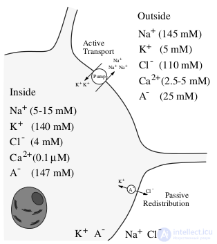 Fig. 2 - Ion composition of the neuron and the environment
 In addition to the pumps, there are ion channels on the surface of the neuron, which, when the potential changes or under chemical action, can open or close, thereby increasing or decreasing the currents of a certain type of ion. If the membrane potential exceeds a certain threshold, sodium channels open, and since there is more sodium outside, an electric current directed inside the neuron arises, which further increases the membrane potential and opens the sodium channels even more, a sharp increase in the membrane potential occurs, physicists call it a positive reverse connection. But starting from some potential value higher than the threshold potential of opening sodium channels, potassium channels are also opened, due to which potassium ions begin to flow outwards reducing the membrane potential, thereby returning it to the equilibrium value. If the initial excitation is less than the threshold for opening sodium channels, then the neuron will return to its equilibrium state. Interestingly, the amplitude of the generated pulse weakly depends on the amplitude of the exciting current, or the pulse exists or is absent, the “all or nothing” law. This is graphically illustrated in Figure 3. The input current below is directed to the inner side of the neuron's membrane, and at the top is the potential difference between the inner and outer side of the membrane. Therefore, according to the currently dominant concept in living neural networks, information is encoded in the times when pulses arise, or as physicists would say, by phase modulation.
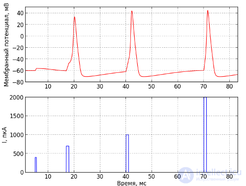 Fig. 3 - The generation of nerve impulses. The bottom shows the current supplied to the cell in the PCA, and at the top is the membrane potential in mV
 It is possible to excite a neuron, for example, by inserting a microelectrode into it and applying current to the inside of the neuron, but in the living brain, the excitation usually occurs via synaptic influence. As already mentioned, neurons are connected to each other using synapses, which are formed at the points of contact of the axon of one neuron with the dendrites of the other. The neuron from which the signal goes is called presynaptic, and the one to which the signal goes is postsynaptic. When a pulse arises on a presynaptic neuron, it will isolate neurotransmitters in the synaptic cleft, which open sodium channels on the postsynaptic neuron, and then a chain of events already described above that lead to excitation occurs. In addition to excitation, neurons can also inhibit each other. If the presynaptic neuron is inhibitory, it will release the inhibitory neurotransmitter opening the chlorine channels into the synaptic cleft, and since there is more chlorine outside, chlorine flows into the neuron because of which the negative charge on the inner side of the membrane increases (do not forget that chlorine ions in differences from sodium and potassium are negatively charged), driving the neuron to an even more inactive state. In this state, the neuron is more difficult to excite.
Mathematical model of neuron
Based on the above-described dynamic mechanisms of the neuron, its mathematical model can be compiled. At the moment, various are created as relatively simple models, like “Inregrate and Fire”, in which the neuron is represented as a capacitor and a resistor. Similarly, more complex, biologically plausible, models, such as the Hodgkin-Huxley model, which is much more complicated both computationally and in terms of analyzing its dynamics, but it describes the dynamics of the membrane potential of a neuron much more accurately. In this article, we will use the Izhikevich model [1]; this model is a compromise between computational complexity and biophysical plausibility. Despite its computational simplicity, this model can reproduce a large number of phenomena occurring in real neurons. The Izhikevich model is defined as a system of differential equations which are depicted in Figure 4.
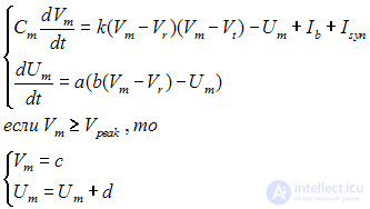 Fig. 4 - Izhikevich model
 Where
a, b, c, d, k, Cm are different parameters of the neuron.
Vm is the potential difference on the inside and outside of the membrane, and
Um is the auxiliary variable.
I is the external direct current applied. In this model, such neuron-specific properties are observed as: spike generation in response to a single external current pulse and generation of a spike sequence with a certain frequency when a constant external current is applied to a neuron.
Isyn is the sum of synaptic currents from all neurons with which this neuron is connected.
If a spike is generated on a presynaptic neuron, a synaptic current jump occurs on the postsynaptic neuron, which exponentially decays with a characteristic time.
Go to coding
So, we get down to the most interesting, it's time to code a virtual piece of nervous tissue on a computer. For this, we will numerically solve a system of differential equations defining the dynamics of the membrane potential of a neuron. For the integration we will use the Euler method. We will code in C ++, draw using scripts written in Python using the Matplolib library, but those who do not have Python can also draw with Exel.
To do this, we will need two-dimensional arrays
Vms, Ums of Tsim * Nneur dimension for storing membrane potentials and auxiliary variables of each neuron, at each moment in time,
Tsim is the simulation time in readings, and
Nneur is the number of neurons in the network.
Links will be stored as two arrays of
pre_con and
post_con of the dimension
Ncon , where the indices are the numbers of the links, and the values are the indices of presynaptic and postsynaptic neurons.
Ncon is the number of connections.
We also need an array to represent the variable modulating the exponentially decaying postsynaptic current of each synapse, for this we create an array
y of the dimension
Ncon * Tsim .
const float h = .5f; // временной шаг интегрирования в мс const int Tsim = 1000/.5f; // время симуляции в дискретных отсчетах const int Nexc = 100; // Количество возбуждающих (excitatory) нейронов const int Ninh = 25; // Количество тормозных (inhibitory) нейронов const int Nneur = Nexc + Ninh; const int Ncon = Nneur*Nneur*0.1f; // Количество сязей, 0.1 это вероятность связи между 2-мя случайными нейронами float Vms[Nneur][Tsim]; // мембранные потенциалы float Ums[Nneur][Tsim]; // вспомогательные переменные модели Ижикевича float Iex[Nneur]; // внешний постоянный ток приложенный к нейрону float Isyn[Nneur]; // синаптический ток на каждый нейрон int pre_conns[Ncon]; // индексы пресинаптических нейронов int post_conns[Ncon]; // индексы постсинаптических нейронов float weights[Ncon]; // веса связей float y[Ncon][Tsim]; // переменная модулирующая синаптический ток в зависимости от спайков на пресинапсе float psc_excxpire_time = 4.0f; // характерное вермя спадания постсинаптического тока, мс float minWeight = 50.0f; // веса, размерность пкА float maxWeight = 100.0f; // Параметры нейрона float Iex_max = 40.0f; // максимальный приложенный к нейрону ток 50 пкА float a = 0.02f; float b = 0.5f; float c = -40.0f; // значение мембранного потенциала до которого он сбрасываеться после спайка float d = 100.0f; float k = 0.5f; float Vr = -60.0f; float Vt = -45.0f; float Vpeak = 35.0f; // максимальное значение мембранного потенциала, при котором происходит сброс до значения с float V0 = -60.0f; // начальное значение для мембранного потенциала float U0 = 0.0f; // начальное значение для вспомогательной переменной float Cm = 50.0f; // электрическая ёмкость нейрона, размерность пкФ
As already mentioned, the information is encoded in the time of occurrence of pulses, so we create arrays to save the time of their occurrence and the indices of neurons where they originated. Then they can be written to a file for visualization purposes.
float spike_times[Nneur*Tsim]; // времена возникновения спайков int spike_neurons[Nneur*Tsim]; // индексы нейронов на которых происходят спайки int spike_num = 0; // номер спайка
We scatter randomly links and set weights.
void init_connections(){ for (int con_idx = 0; con_idx < Ncon; ){ // случайно выбираем постсипантические и пресинаптические нейроны pre_conns[con_idx] = rand() % Nneur; post_conns[con_idx] = rand() % Nneur; weights[con_idx] = (rand() % ((int)(maxWeight - minWeight)*10))/10.0f + minWeight; if (pre_conns[con_idx] >= Nexc){ // если пресинаптический нейрон тормозный то вес связи идет со знаком минус weights[con_idx] = -weights[con_idx]; } con_idx++; } }
Setting the initial conditions for neurons and the random setting of the external applied current. Those neurons for which the external current exceeds the spike generation threshold will generate spikes at a constant frequency.
void init_neurons(){ for (int neur_idx = 0; neur_idx < Nneur; neur_idx++){ // случайно разбрасываем приложенные токи Iex[neur_idx] = (rand() % (int) (Iex_max*10))/10.0f; Isyn[neur_idx] = 0.0f; Vms[neur_idx][0] = V0; Ums[neur_idx][0] = U0; } }
The main part of the program with the integration of Izhikevich model.
float izhik_Vm(int neuron, int time){ return (k*(Vms[neuron][time] - Vr)*(Vms[neuron][time] - Vt) - Ums[neuron][time] + Iex[neuron] + Isyn[neuron])/Cm; } float izhik_Um(int neuron, int time){ return a*(b*(Vms[neuron][time] - Vr) - Ums[neuron][time]); } int main(){ init_connections(); init_neurons(); float expire_coeff = exp(-h/psc_excxpire_time); // для экспоненциально затухающего тока for (int t = 1; t < Tsim; t++){ // проходим по всем нейронам for (int neur = 0; neur < Nneur; neur++){ Vms[neur][t] = Vms[neur][t-1] + h*izhik_Vm(neur, t-1); Ums[neur][t] = Ums[neur][t-1] + h*izhik_Um(neur, t-1); Isyn[neur] = 0.0f; if (Vms[neur][t-1] > Vpeak){ Vms[neur][t] = c; Ums[neur][t] = Ums[neur][t-1] + d; spike_times[spike_num] = t*h; spike_neurons[spike_num] = neur; spike_num++; } } // проходим по всем связям for (int con = 0; con < Ncon; con++){ y[con][t] = y[con][t-1]*expire_coeff; if (Vms[pre_conns[con]][t-1] > Vpeak){ y[con][t] = 1.0f; } Isyn[post_conns[con]] += y[con][t]*weights[con]; } } save2file(); return 0; }
The full text of the code can be downloaded here. The code is freely compiled and run even under Windows with Visual Studio 2010 Express Edition or MinGW, even under GNU / Linux with GCC. Upon completion, the program saves the raster activity, times and indices of the appearance of nerve impulses, and oscillograms of the average membrane potential in the rastr.csv and oscill.csv files, respectively. You can directly them in Exel and draw. Or with the help of the Python scripts attached by me, but for their work the Matplotlib library is needed. For those with GNU / Linux, installing the python-matplotlib package from the repositories is easy, while Windows users will have to manually download the numpy, scypy, pyparsing, python-dateutil and matplotlib packages from here.
Drawing an activity raster - plot_rastr.py
Drawing the average membrane potential - plot_oscill.py
results
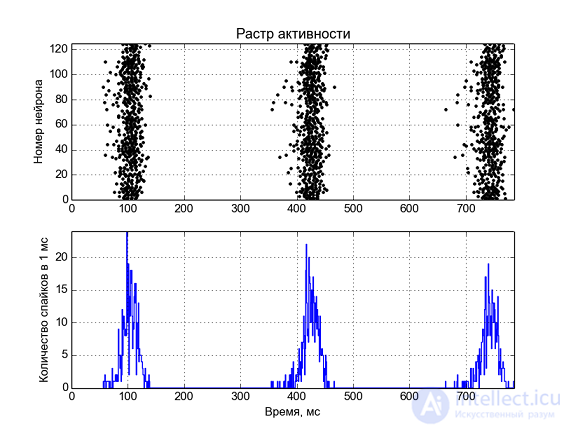 Fig. 5 - Neural network activity. At the top along the y axis the numbers of neurons are plotted, and the points in time when a spike is generated on the neuron are marked with a dot. Below, the average number of spikes in 1 ms time.
 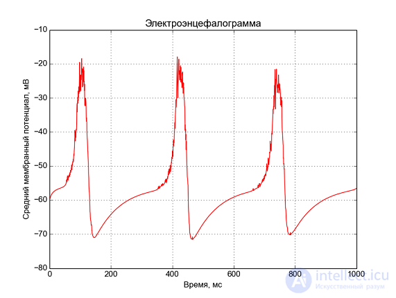 Fig. 6 - Median membrane potential, “electroencephalogram”.
 This is what happens when simulating 1 second of activity of 125 neurons. We observe periodic activity at a frequency of ~ 3 Hz, similar to a delta rhythm.
[1] EM Izhikevich, Dynamic Systems in Neuroscience: The Geometry of Excitability and Bursting, USA, MA, Cambridge: The MIT Press., 2007 
Comments
To leave a comment
Models and research methods
Terms: Models and research methods