Imagine a situation when you need to calculate the signal-to-noise ratio at the output row devices of known frequency bandwidth, but different gains. After all, this ratio determines, as a result, the probability of detecting a signal. and false alarm. It is necessary to calculate each time the signals at the output and the noise of all the stages, taking into account the amplification of the subsequent ones. It is rather laborious and inconvenient. Therefore, instead of this, the level of conditional, so-called “reduced” noise to the input is calculated . In this case, the device is considered not to be noisy, and the input level is such that, at the output, the calculated noises turn out to be, as in a real product.
This is convenient, since the signal-to-noise ratio at the input and output will no longer depend on the gain. Moreover, considering the input noise as “white”, it is possible to extrapolate the power spectral density over a wide range of frequencies and then use it to calculate ratios for any linear devices. The stated considerations are illustrated in fig. 2.4 for example video amplifier (MAS)
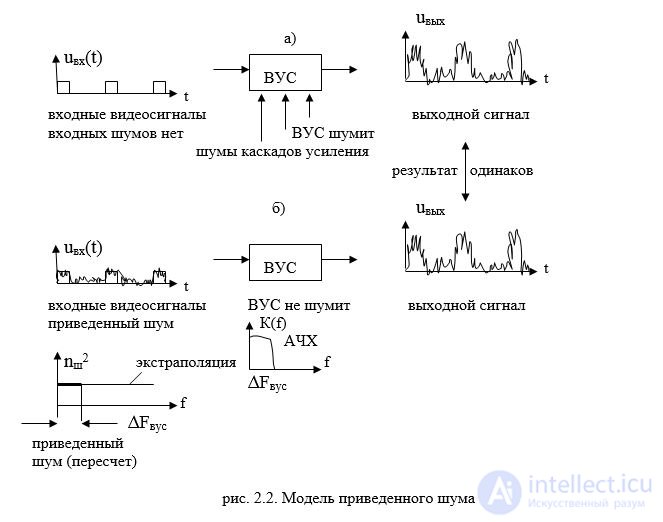
rice 2.2. Reduced noise model
The power calculation of the “reduced” noise is considered in several ways.
From reference books, the noise temperature of a radio engineering device of this type T W is known . Then you can calculate the desired value from equations (1).
Often known is the temperature of the receiver input circuits and its noise figure. Then the method of claim 1. is modified.
Sometimes directly indicated The spectral density of the reduced noise n Ш 2 for this type of device , for example, 10 -18 W / Hz. Then it is easy to calculate the “reduced” to the input noise power pw , multiplying this value by ? F.
Real measurements on the sample.
So, the first 3 ways :
p w = k b T sh ? F
N w = [ p with / p w ] in / [ p s / p w ] o , p w = N w k b T sh ? F ; (2)
p w = n w 2 ? F
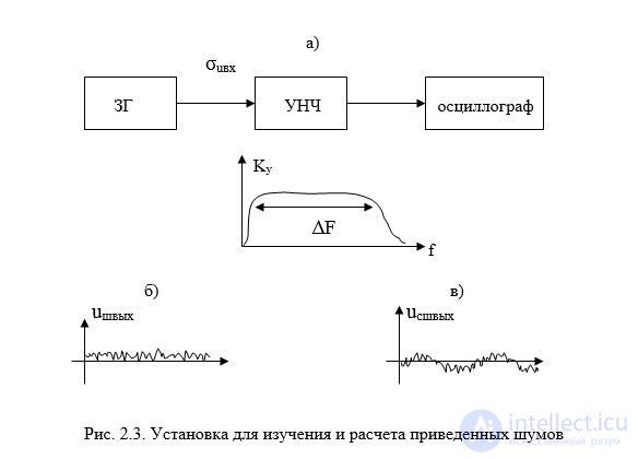
Practical measurements and calculation of reduced noise are made as follows. Let's give an example explained in fig. 2.3 for low frequency amplifier. (ULF)
Fig. 2.3. Installation for the study and calculation of reduced noise
Laboratory work, the principle of which is shown in Fig. 2.3 allows you to understand the meaning model “reduced” noise and calculate the approximate value of the extrapolated power spectral density. The procedure for working with the installation of the following.
Assemble the setup, consisting of a sound generator with an accurate display of the input signal, a low-frequency amplifier and an oscilloscope.
Take the amplitude - frequency response and measure the gain K y on the central part and the bandwidth ? F.
3 Observing on an oscilloscope, the input signal level is reduced to a value when the amplitude of the sinusoid is approximately equal to the noise level. Measure the input signal level ( ? U with ) in x on the GG scale, taking into account the attenuator values.
Next, make recounts
( ? u sh ) in x = ( ? u c ) in , p w = ( ? u w ) in 2 , n sh 2 = p sh /? F (3)
If for some reason it was not possible to assemble the diagram in fig. 2.3, but the gain and the bandwidth are known. It is enough to measure the noise level at the output ( ? U sh ) in s . Then:
p w = [ ( ? u w ) in s / K y ] 2 , n w 2 = p w /? F (four)

Comments
To leave a comment
Radio Engineering Systems
Terms: Radio Engineering Systems