5. Quantification of software reliability

5.1. Quality characteristic of software "Reliability" according to ISO 9126

The international standard ISO / IEC 9126 defines 6 basic characteristics of software quality: functionality, reliability, practicality, efficiency, maintainability, portability. To characterize the reliability, 4 sub-characteristics are defined: completeness, fault tolerance, recoverability and consistency of reliability.

Metrics for sub-characteristics:

Completion metrics:
1.1. fault detection shows how many errors were detected during the examination of the product;

1.2. troubleshooting - shows the number of corrected errors;

1.3. test adequacy - shows how the required test effects are covered by the test plan.

Failover Metrics:
2.1. fault avoidance — shows the number of fault patterns that were brought under control to avoid emergency and critical faults;

2.2. invalid avoid operation - the number of functions implemented to avoid invalid schemes of operations.

Recoverability metrics:
3.1. recoverability - shows how the product is able to recover from an unforeseen event or request;

3.2. recovery efficiency - how effective is the ability to recover.

Reliability Compliance Metrics:
4.1. compliance reliability — indicates how well the product complies with the applicable provisions of the standards.

5.2. Quantifying software reliability using the Harrington-Mencher function

5.2. Quantifying software reliability using the Harrington-Mencher function

The prerequisites for the creation of this assessment methodology were the lack of a convenient approach for processing the calculated values ​​of metrics. It is based on several concepts. Consider them in order.

The value of each reliability metric (see § 5.1.) Is converted to a dimensionless desirability scale d , also called the Harrington desirability scale. Thus, the physical parameter, which is the metric, is converted into a psychological value, which is a numerical expression of the empirical evaluation of this metric.

It reflects the opinion of an observer (he is a programmer, analyst, expert - in general, it is a certain person whose object of consideration is the reliability of this software product) and is in the interval from zero to one. A zero value corresponds to an absolutely unacceptable level of this property, a single value to the best. The ratio between the values ​​of the desirability scale in the empirical and numerical (psychological) systems is presented in table 5.1.

Table 5.1. - The relationship between the quantitative values ​​of the dimensionless scale and the psychological perception of a person

The choice of marks on the desirability scale of 0.63 and 0.37 is dictated by the convenience of calculations: 0.63 ~ = 1- (1 / e), 0.37 ~ = 1 / e. The value of d i = 0,37 corresponds to the limit of acceptable values.

Such an approach implies the choice of the function defining the considered transformation, the desirability function . It can be calculated by the formula

, (5.1)

where d is the value on the scale of desirability

y is the initial value of the metric.

To calculate the quantitative assessment of the reliability of a software product, we will use the generalized desirability function of Harrington-Mencher:

D   = , (5.2.)

Where D k   - generalized desirability function for the k -th sub-characteristic, having weight а k ;

4 - the number of subcharacteristics.

Each sub-characteristic of reliability, in turn, can be represented as a function:

D k = , (5.3)

where d i   - private function of desirability of i - th metric , having weight a i i ;

m is the number of metrics in a given sub-characteristic.

The calculation is made in two stages.

At the first stage, single values ​​of the function d i ( i = 1, 2, ..., m ) are determined for any number of responses, each of which must represent a continuous monotonic function. For the case of increasing quality with increasing numerical values ​​of the response, 3 types of dependencies were proposed (types 1, 2 and 3 in Fig. 5.1), and for the case of decreasing quality with increasing numerical values ​​of the response, three more types of dependencies were proposed (types 4, 5 and 6 in Fig. .5.2). In this case, in all cases, the argument is the response Y   in its natural form - as it was measured during the experiment, this is a great advantage for the method of calculation.

Figure 5.1. - Graphs of the desirability functions of the three increasing types

For all three types of ascending curves, the correct purpose of the beginning of b and the end of   the physical (or acceptable) value of the response Y , that is, the condition

(5.4)

In this case, the curve of type 1 is S- shaped, increasing, symmetric and describes the quality of the response Y , if the distribution of Y is not sharply asymmetric, according to the formula

. (5.5)

The curve type 2 is S- shaped, increasing, asymmetric with a rapid initial increase and is calculated by the formula

, (5.6)

where the exponent a II determines the rate of increase of the function d . To calculate it, you need to know (or specify) at least one point ( Y II ; d II ) on the desired graph. Then the value of a II can be calculated by the formula

. (5.7)

Similarly, a type 3 curve is S- shaped, increasing, asymmetric with a slow initial increase and is calculated by the formula

, (5.8)

where the exponent a III can be found by a single point ( Y III ; d III ) by the formula

. (5.9.)

Figure 5.2 - Graphs of the desirability functions of three decreasing types

For all three types of decreasing curves, the correct purpose of the beginning e and the end f of the physical (or permissible) value of the response Y is decisive, that is, the condition

(5.10)

The type 4 curve is S- shaped, decreasing, symmetric, is a mirror version of the type 1 curve, and is described by the formula

. (5.11)

The type 5 curve is S- shaped, decreasing, asymmetric, with a rapid initial decrease, is a mirror version of the type 3 curve, and is described by the formula

, (5.12)

where the exponent a V determines the rate of decrease of the function d . To calculate it, you need to know (or specify) at least one point ( Y V ; d V ) on the desired graph. Then the value of a V can be calculated by the formula

. (5.13)

Similarly, the curve of type 6 is S- shaped, decreasing, asymmetric, with a slow initial decrease, is a mirror version of the curve of type 2, and is described by the formula

, (5.14)

where the exponent a VI can be found by a single point ( Y VI ; d VI ) by the formula

. (5.15)

If we assume that quantitative samples have a normal distribution law (Fig. 5.3), then we obtain the following formulas for calculating the partial indicators of the quality of metrics d i :

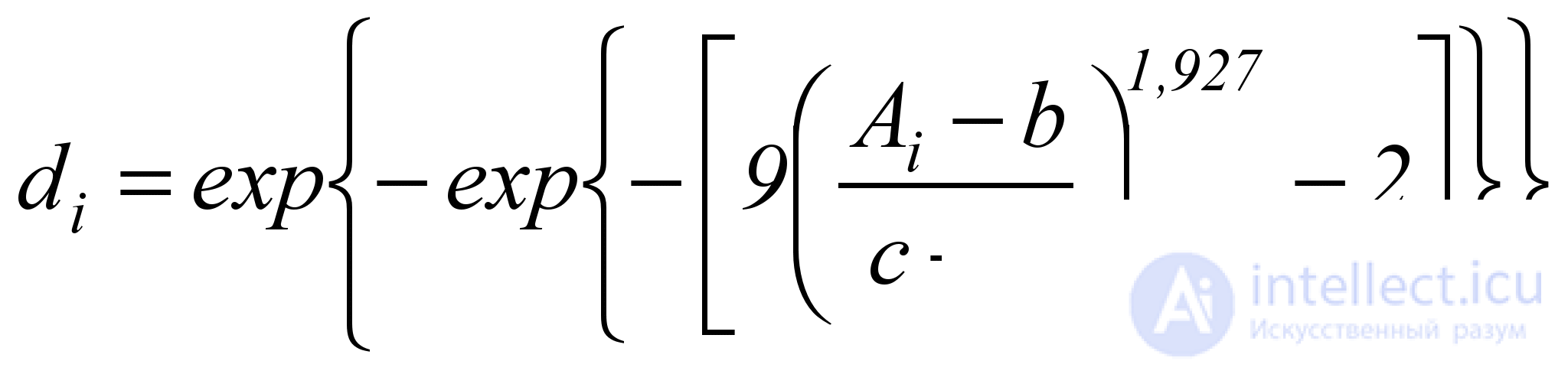, (5.16)

where d i is the quality indicator of the i -th metric;

A i - the real value of the i -th metric;

b - the minimum possible value of the i -th metric;

c - the maximum possible value of the i -th metric.

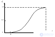
Figure 5.3 - Normal distribution of samples

After calculating the specific indicators of the quality of metrics, a generalized quality function is calculated for each sub-characteristic (according to formula 5.3). A feature of this calculation is the preliminary finding for each particular indicator d i of its weight a i . To determine the weights of particular indicators of quality a i , the method of weighting coefficients of importance (CKB) is used. Programmers fill out questionnaires in which they evaluate the significance of each metric (an example of the questionnaire in Figure 5.4).

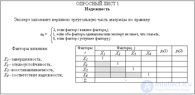
Figure 5.4 - an example of a questionnaire to be filled by experts when using the method VKB

The ranking of objects of comparison using expert methods necessarily includes a procedure for checking the correctness of the results obtained. For this, the following 4 steps are used in the weighting importance coefficient method:

1. The coefficient of internal consistency of the answers of each expert is calculated. If this coefficient is less than 0.5, then the expert’s opinion is discarded;

2. To assess the homogeneity of opinions on each particular object, Cochren's criterion is applied;

3. The coefficient of concordance is calculated, which shows the degree of homogeneity of expert opinions;

4. If different groups of experts give conflicting answers to the same questions, then Zipf's law applies.

Then, according to formula 5.2, a quantitative estimate of the reliability of the software product is calculated (for each sub-characteristic of reliability, the weights a k   using the method VKB)