Lecture
Topic 5. Regular methods for constructing binary error-correcting codes.
Lecture 7 .
7.1 Line codes. General construction methods.
Consider the class of noise-tolerant algebraic codes, called linear or often linear group.
Definition: Linear codes are block codes, the additional bits of which are formed by linear operations on information bits.
The concept of linear operation is used here. In coding theory, modulo 2 (+) addition is used as a linear addition operation.
7.2 Determination of the number of additional digits r.
To determine the number of additional digits, we can use the Hamming boundary formula already known to us:
<! [if! vml]> 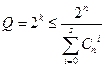 <! [endif]>
If s = l, that is, a code is built that corrects a maximum of one-time errors, then:
<! [if! vml]>  <! [endif]> ,
where do we get
2 r ≥r + k
Taking into account the last formula, the smallest r is sought at which this inequality is satisfied.
Example: n = 7, then it is easy to find by simple enumeration that r = 3 . And the corresponding code is of the form n (7,4).
7.3 Construction of the generating (generating) matrix | OM |.
Linear codes have the following property:
- from the whole set of 2 k allowed code words that form a linear group, we can distinguish subsets of k words with the property of linear independence.
Linear independence means that none of the words in a subset of linearly independent code words can be obtained by summing (using a linear expression) any other words in this subset.
At the same time, any of the allowed codewords can be obtained by summing certain linearly independent words.
Thus, the construction of code combinations of a linear code is associated with linear operations. To perform such operations, it is convenient to use a well-developed apparatus of matrix calculations.
To form n- bit code words from k-bit coded words (coding), a matrix is used, which is called a generator (generator).
The generator matrix is obtained by writing to the column k linearly independent words.
Denote the encoded information sequence X and write it in the form of a matrix-row || X || dimension 1 * k , for example:
|| X || = || 11001 ||, where k = 5 .
One of the methods for constructing a generator (generating) matrix is as follows: It is built from the unit matrix || I || of dimension k * k and the matrix of additional (redundant) digits assigned to it on the right || dimension k * r .
<! [if! vml]> 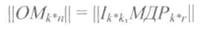 <! [endif]>
where at k = 4
<! [if! vml]> 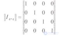 <! [endif]>
This structure OM provides systematic code.
The order of construction of the MDR matrix will be discussed below.
7.4 Encoding procedure.
The code word KS is obtained by multiplying the matrix of the information sequence || X || on the generating matrix || OM ||:
<! [if! vml]> 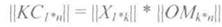 <! [endif]>
Multiplication is performed according to the rules of matrix multiplication: (so it is)
<! [if! vml]> 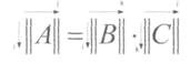 <! [endif]>
It is necessary only to remember that the addition is here modulo 2.
Example:
let's say the generator matrix
1000 110
0100 111
|| OM || = 0010 011
0001 101
and row vector information sequence
<! [if! vml]>  <! [endif]> .
Since the multiplicand matrix has only one row, multiplication is simplified. In this case, you should put in correspondence to the rows of the generator (generating) matrix || ОМ || digits of the information sequence matrix || X || and add those rows of the generator (generating) matrix, which correspond to the unit digits of the matrix || X ||.
<! [if! vml]> 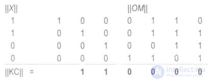 <! [endif]>
Note that || KC || = || X, DR ||,
where || X || is the information sequence (since it is multiplied by the unit matrix || I || ),
a || dr || - additional discharges depending on the matrix of additional discharges || MDR || :
|| DR || = || X || * || MDR ||
7.5 Decoding Order.
As a result of a code word being transmitted through a channel, it may be distorted by interference. This will lead to the fact that the adopted code word || PKS || may not coincide with the original || KS ||.
Distortion can be described using the following formula:
|| PKS || = || COP || + || VO ||,
where || into || - the error vector is a matrix-row of 1 * n dimension, with 1 in those positions where distortions have occurred.
Decoding is based on finding the so-called identifier or error syndrome -matrix-strings || OP || length r bits ( r - the number of additional or redundant bits in the code word).
The identifier is used to find the estimated error vector.
The identifier is found according to the following formula:
|| OP || = || PKS || * || SST ||,
where || PKS || is an adopted and possibly distorted code word;
|| TPM ||, - transposed test matrix, which is obtained from the matrix of additional digits || MDR || by assigning to it from below the identity matrix:
<! [if! vml]> 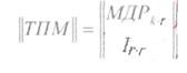 <! [endif]>
Example || TPM ||:
<! [if! vml]> 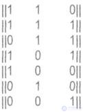 <! [endif]>
Since || PKS || = || COP || + || BO ||, the last formula can be written as:
|| OP || = || COP || * || TPM || + || IN || * || TPM ||.
Consider the first term.
|| KC || - matrix-row, with the first k bits - informational.
We now prove that the product of the code word || KS || on || TPM || results in the zero matrix || 0 ||.
Since || cop || - matrix-row, it is possible to simplify the multiplication of the matrices discussed above.
<! [if! vml]>  <! [endif]>
Therefore, the first term in
|| OP || = || COP || * || TPM || + || VO || * || TPM ||
always equal to zero and the identifier completely depends on the error vector || VO ||.
If we now select such a verification matrix of the SST , and therefore the MDR , so that different PD identifiers correspond to different error vectors , then these identifiers will be able to find the error vector of the VO, and therefore correct these errors.
The correspondence of the identifiers to the error vectors is found in advance by multiplying the vectors of corrected errors on the SST;
<! [if! vml]>  <! [endif]>
Thus, the code's ability to correct errors is entirely determined by || MDR ||. To build an MDR for codes that correct one-time errors, you need to have at least 2 units in each MDR line. It is also necessary to have at least one difference between any two lines of MDR .
The code we received is inconvenient because the identifier, although it is uniquely associated with the number of the distorted digit, as the number is not equal to it. To search for a distorted digit, you need to use an additional table of correspondence between the identifier and this number. Codes in which the identifier as a number determines the position of the distorted digit were found and called Hamming codes .
Building an MDR for the case of correcting multiple errors is much more complicated. Different authors have found various algorithms for constructing || MDR || for this case, and the corresponding codes are called the names of their authors.
7.6 Systematic codes. Hamming code.
Systematic codes are such codes in which informational and corrective bits are located on a strictly defined system and always occupy strictly defined places in code combinations.
Systematic codes are uniform, that is, all combinations of a code with given corrective abilities have the same length. Systematic codes can be constructed as linear on the basis of the generating matrix, as has already been considered.
Usually the generating matrix is constructed using two matrices:
Single, the rank of which is determined by the number of information bits, and additional, the number of columns is determined by the number of control bits of the code. Each row of the additional matrix must contain at least d 0 -1 units, and the modulo sum for any rows must be at least d 0 -2 units (where d 0 is the minimum code distance).
The generating matrix allows to find all other code combinations.
The Hamming code is a typical example of a systematic code. However, in its construction, matrices are usually not resorted to. It is so well studied that it has already developed a clear algorithm for its construction:
The Hamming code is one of the most important classes of linear codes that are widely used in practice and have a simple and convenient for technical implementation algorithm for detecting and correcting errors.
The ratios between n, r, k for the Hamming code are presented in the table. Knowing the basic parameters of the correction code, they determine which positions of the signals will be working and which - control. Practice has shown that the numbers of control characters are conveniently chosen by law.
2 i , where i = 0, 1, 2, 3, ... is a natural series of numbers.
The numbers of control symbols in this case are 1, 2, 4, 16, 32 ... Then the values of the control coefficients ( 0 or 1 ) are determined, guided by the following rule:
the sum of the units in the test positions must be even. If this sum is even the value of the control coefficient is zero, otherwise it is one.
Relations between the number of information and control characters in the Hamming code
Table 7.1
<! [if! vml]> 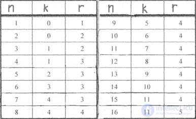 <! [endif]>
Test items are selected as follows. Make up the plate for a number of natural numbers in binary code. The number of rows is n = r + k. The first line corresponds to the test coefficient a 1 , the second and 2, and so on:
<! [if! vml]>  <! [endif]>
Then identify the test position, writing out the coefficients according to the following principle:
The first check includes coefficients that contain a one in the low order ( a 1 , a 3 , a 5 , a 7 , a 9 , a 11 , etc.);
in the second - in the second digit ( a 2 , a 3 , a 5 , a 7 , a 9 , a 11 , etc.);
in the third - in the third digit, etc.
The numbers of the verification coefficients correspond to the numbers of the verification positions, which allows you to create a general table of checks.
Non checkout numbers of the Hamming code
Table 7.2
<! [if! vml]>  <! [endif]>
Hamming code generation
Example: Build the layout of the Hamming code and determine the values of the correction bits for the code combination k = 4, X = 0101 .
Table 7.3
<! [if! vml]>  <! [endif]>
Decision:
According to the table, the minimum number of control symbols is r = 3 , with n = 7 . The control coefficients will be located at positions 1, 2, 4. We compose a model of the correction code and write it in the second column of the table. Using the table for the numbers of test coefficients, we determine the values of the coefficients K1 K2 and K3 .
The first check: the sum P1 + P3 + P5 + P7 should be even, and the sum K1 + 0 + 1 + 1 will be even when K = 0.
The second check: the sum P2 + P3 + P6 + P7 should be even, and the sum K2 + 0 + 0 + 1 will be even with K2 = 1.
The third check: the sum of P4 + P5 + P6 + P7 should be even, and the sum of K3 + 1 + 0 + 1 will be even with K3 = 0.
The final value of the desired combination of the correction code is recorded in the third column of the code layout table.
7.7 Detection and correction of errors in the Hamming code.
An example . Suppose a distortion occurred in the communication channel under the influence of interference and 0100101 (01) 1 was taken instead of 0100101.
Solution : For detecting errors, parity checks already known to us are produced.
First check : the sum of П1 + П3 + П5 + П7 = 0 + 0 + 1 + 1 is even. In the lower digit of the error position number, we write 0.
The second check : the sum П2 + П3 + П6 + П7 = 1 + 0 + 1 + 1 is odd. In the second digit of the error position number, we write 1
The third check : the sum of P4 + P5 + P6 + P7 = 0 + 1 + 1 + 1 is odd. In the third digit of the error position number, we write 1. The error position number 110 = 6 . Therefore, the symbol of the sixth position should be reversed, and we will get the correct code combination.
Code correcting single and detecting double errors
Table 7.4
<! [if! vml]> 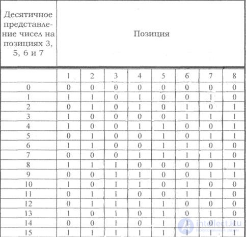 <! [endif]>
If, according to the above rules, to build a correction code with the detection and correction of a single error for a uniform binary code, then the first 16 code combinations will have the form shown in the table. Such code can be used to build a code with a single error correction and double detection.
For this, in addition to the above checks on control positions, one more parity check should be carried out for the entire line as a whole. To carry out such a check, add to each line of the code the control characters recorded in the additional column (table, column 8). Then, in the case of one error, the check on positions will indicate the number of the error position, and the even check will indicate the error. If the position checks indicate the presence of an error, and the parity check does not fix it, then there are two errors in the code combination.
7.8 Test questions.
1. A general method for constructing a linear code.
2. Requirements for generating matrix.
3. What is the TPM verification matrix?
4. What is the advantage of the Hamming coding method?
5. How many errors can fix Hamming code

Comments
To leave a comment
Information and Coding Theory
Terms: Information and Coding Theory