Lecture
Topic 9 . Coding methods with compression and loss of information .
15 1 Compression methods with loss of information.
As previously noted, there are two types of data compression systems:
· lossless information
· loss of information
When lossless coding, the original data can be recovered from compressed in its original form, that is, absolutely accurate. Such encoding is used for compressing texts, databases, computer programs and data, etc., where even the slightest difference is unacceptable. All the encoding methods discussed above were related to lossless encoding.
Unfortunately, compression or lossless coding, when there is a complete coincidence of the original and recovered data, has low efficiency - compression ratios rarely exceed 3 ... 5 (except for cases of data coding with a high degree of repeatability of the same areas, etc.).
15 2 Accuracy . Interference and distortion . Approximate recovery.
Accuracy. However, very often there is no need for absolute accuracy of the transfer of source data to the consumer. First, the data sources themselves have a limited dynamic range and generate source messages with a certain level of distortion and errors. This level may be higher or lower, but absolute fidelity cannot be achieved.
Interference and distortion . Secondly, data transmission over communication channels and their storage are always carried out in the presence of various kinds of interference. Therefore, the received (reproduced) message is always to a certain extent different from that sent, that is, in practice, absolutely accurate transmission is impossible in the presence of interference in the communication channel (in the storage system).
Susceptibility. Finally, messages are transmitted and stored for their perception and use by the recipient. Recipients of the same information - human senses, actuators, etc. - also have a finite resolution, that is, they do not notice a slight difference between the absolutely accurate and approximate values of the reproduced message. The threshold of sensitivity to distortion may also be different, but it always is.
Approximate recovery. Loss coding takes into account these arguments in favor of approximate data recovery and makes it possible to obtain compression ratios, sometimes tens of times greater than the lossless compression methods, at the expense of some controlled error.
Pre-conversion . Most lossy compression methods are based not on the coding of the data itself, but of some linear transformations from them, for example, the Discrete Fourier Transform (DFT) coefficients, cosine transform coefficients, Haar and Walshai transforms, etc.
In order to understand the basis of high efficiency of systems compression with losses and why transformation coding turns out to be much more efficient than source data coding, let's take as an example the popular method of compressing JPEG images (“dzhipeg”), which contains all the necessary signs of compression system with losses. We will not go into the formula thickets now, the main thing is to understand the idea of coding transformations.
It will also be necessary to consider the essence of the linear transformations used for compression, since without an understanding of their physical meaning it is difficult to understand the reasons for the effects obtained.
15 3 Transformation coding . JPEG compression standard .
The popular JPEG (Joint Photographers Experts Group) image encoding standard is a very good illustration of the explanation of the principles of lossy compression based on coding transformations.
To compress lossy graphic information, one standard was set at the end of the 1980s — the JPEG format (Joint Photographic Experts Group — the name of the association of its developers). In this format, you can adjust the degree of compression, setting the degree of loss of quality.
Simple decrease in digit capacity. The basic idea of coding transformations can be understood from the following simple reasoning. Suppose we are dealing with some digital signal (a sequence of Kotelnikov counts). If we discard half of the binary bits in each of the samples (for example, 4 bits out of eight), then the code size R will be halved and half of the information contained in the signal will be lost .
DFT and simple decrease in digit capacity. If we subject the signal to Fourier transform (or some other similar linear transformation), divide it into two components - LF and HF, sample it, quantize each of them and discard half of the binary bits in the high-frequency component of the signal, then the resulting code volume will decrease one third, and the loss of information will be only 5% .
This effect is due to the fact that the low-frequency components of most signals (large parts) are usually much more intense and carry much more information than high-frequency components (small details). This applies equally to audio signals and to images.
Consider the work of the JPEG compression algorithm when encoding a black and white image, represented by a set of its samples (pixels) with the number of gradations of 256 levels (8 binary digits). This is the most common way to store images - each point on the screen corresponds to one byte (8 bits - 256 possible values), which determines its brightness. 255 - maximum brightness (white color), 0 - minimum (black color). Intermediate values make up the rest of the gray range (Fig. 15.1).
<! [endif]> <! [if! RotText]>  <! [endif]> <! [if! vml]>
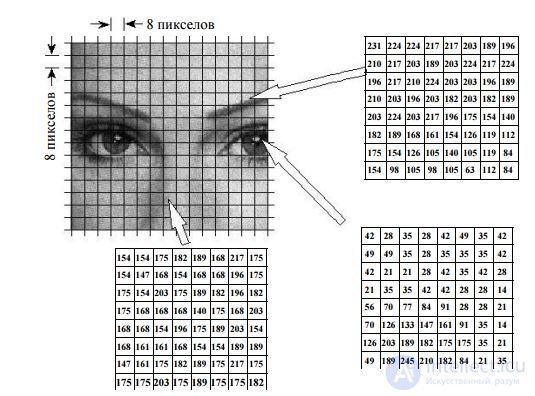
Fig. 15.1
The work of the JPEG compression algorithm begins with splitting the image into square blocks of 8x8 = 64 pixels. Why exactly 8x8, not 2x2 or 32x32? The choice of such a block size is due to the fact that with its small size the effect of compression will be small (with a size of 1x1 it will be completely absent), and with a large size, the image properties within the block will change dramatically and the coding efficiency will decrease again.
In fig. 15.1 depicts several such blocks (in the form of matrices of digital samples) taken from different parts of the image. In the future, these blocks will be processed and encoded independently of each other.
The second stage of compression is applying to all blocks of the discrete cosine transform - DCT . For data compression they tried to apply many different transformations, including specially designed for these purposes, for example, the Karhunena-Loeve transformation, which provides the maximum possible compression ratio. But it is very difficult to implement in practice. Fourier transform is very simple, but does not provide good compression. The choice was stopped on a discrete cosine transform, which is a type of PF. Unlike the PF, which uses sine and cosine frequency components for signal decomposition, only cosine components are used in DCT . The discrete cosine transform allows you to go from the spatial representation of the image (a set of samples or pixels) to the spectral representation (set of frequency components) and vice versa.
Discrete cosine transform from image
IMG (x, y) can be written as follows:
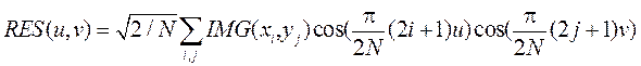
where N = 8.0 <i <7, 0 <j <7,
or, in matrix form,
RES = DCT T * IMG * DCT,
where DCT is the matrix of basic (cosine) coefficients for the 8x8 transformation, has a specific form:
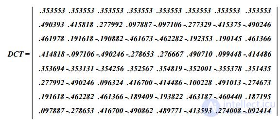
The inverse reconstruction of the matrix of pixels of the original IMG image by its DCT transformation in matrix form has the obvious form:
IMG = DCT * RES * DCT T
So, as a result of applying an 8x8 pixel image to the block, we obtain a two-dimensional spectrum that also has 8x8 samples. In other words, 64 numbers representing image samples will turn into 64 numbers representing samples of its DCT spectrum.
And now we recall that such a signal spectrum. These are the values of the coefficients with which the corresponding spectral components are included in the sum, which as a result gives this signal. The individual spectral components into which the signal is decomposed are often called basic functions. For the Fourier transform, the basic functions are the sines and cosines of different frequencies.
For a 8x8 DCT basis functions system is given by
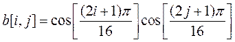 ,
,
The basic functions themselves look like the ones shown in fig. 15.2. for one-dimensional DCT transformation for n = 4, 8, 16. The figure gives us an idea of the quality characteristics of the transformation or decomposition of the input signal into spectral components. By the nature of the behavior of the basis functions, it can be seen that the functions with the lowest numbers extract low-frequency components from the signal spectrum, and as the function number increases, it highlights all the higher-frequency components of the signal.
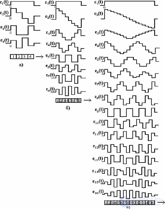
Fig. 15.2
In fig. 15.3 shows the behavior of the basis functions of the two-dimensional DCT for n = 4. It is easy to see that the cross section of each square horizontally coincides with the behavior of one-dimensional DCT for n = 4 for the situation in Fig.15.2
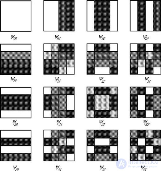
Fig. 15.3
The lowest-frequency basic function corresponding to the indices (0,0) is shown in the upper left corner of the figure, the highest-frequency function in the lower right. The base function for (0,1) is the half of the cosinusoid period in one coordinate and the constant in the other, the base function with indices (1.0) is the same, but rotated by 90 0 .
The discrete cosine transform is computed by element-wise multiplying and summing the image blocks of 8x8 pixels with each of these basis functions. As a result, for example, the component of the DCT spectrum with indices (0,0) will simply be the sum of all the elements of the image block, that is, the average brightness for the block. In the component with the index (0,1), all horizontal image details are averaged with the same weights, and vertically the elements of the upper part of the image, etc., are assigned the greatest weight. You can see that the lower and to the right in the DCT matrix of its component, the more high-frequency details of the image it corresponds to.
In order to get the original image from its DCT spectrum (perform the inverse transformation), you now need to multiply the base function with indices (0,0) by the spectral component with coordinates (0,0), add the product of the base function (1, 0) on the spectral component (1.0), etc.
In the table below. 15.1 shows the numerical values of one of the image blocks and its DCT spectrum:
Table 15.1
Initial data | |||||||
139 | 144 | 149 | 153 | 155 | 155 | 155 | 155 |
144 | 151 | 153 | 156 | 159 | 156 | 156 | 156 |
150 | 155 | 160 | 163 | 158 | 156 | 156 | 156 |
159 | 161 | 161 | 160 | 160 | 159 | 159 | 159 |
159 | 160 | 161 | 162 | 162 | 155 | 155 | 155 |
161 | 161 | 161 | 161 | 160 | 157 | 157 | 157 |
161 | 162 | 161 | 163 | 162 | 157 | 157 | 157 |
162 | 162 | 161 | 161 | 163 | 158 | 158 | 15 |
DCT result | |||||||
235.6 | -one | -12,1 | -5.2 | 2.1 | -1,7 | -2,7 | 1,3 |
-22,6 | -17,5 | -6,2 | -3,2 | -2.9 | -0,1 | 0.4 | -1,2 |
-10.9 | -9.3 | -1,6 | 1.5 | 0.2 | -0.9 | -0,6 | -0,1 |
-7.1 | -1.9 | 0.2 | 1.5 | 0.9 | -0,1 | 0 | 0.3 |
-0,6 | -0,8 | 1.5 | 1.6 | -0,1 | -0.7 | 0.6 | 1,3 |
1.8 | -0,2 | 1.6 | -0,3 | -0,8 | 1.5 | one | -one |
-1.3 | -0,4 | -0,3 | -1.5 | -0.5 | 1.7 | 1.1 | -0,8 |
-2,6 | 1.6 | -3,8 | -1.8 | 1.9 | 1.2 | -0,6 | -0,4 |
We note a very interesting feature of the obtained DCT- spectrum: its largest values are concentrated in the upper left corner of the table. 15.1 (low-frequency components), the right lower part (high-frequency components) is filled with relatively small numbers. These numbers, however, are the same as in the image block: 8x8 = 64, that is, so far no compression has taken place, and if we perform the inverse transform, we get the same image block.
The next stage of the JPEG algorithm is quantization (Table 15.2).
If you look closely at the resulting DCT coefficients, it will be seen that a good half of them are zero or have very small values (1 - 2). These are high frequencies, which (usually) can be painlessly dropped or at least rounded to the nearest integer value.
Quantization consists in dividing each DCT coefficient by a certain number in accordance with the quantization matrix. This matrix can be fixed or, for better and more efficient compression, obtained by analyzing the nature of the original image. The greater the number into which division occurs, the greater the result of the division will be zero values, which means stronger compression and more noticeable loss.
Table 15.2
Previously obtained DCT result | |||||||
235.6 | -one | -12,1 | -5.2 | 2.1 | -1,7 | -2,7 | 1,3 |
-22,6 | -17,5 | -6,2 | -3,2 | -2.9 | -0,1 | 0.4 | -1,2 |
-10.9 | -9.3 | -1,6 | 1.5 | 0.2 | -0.9 | -0,6 | -0,1 |
-7.1 | -1.9 | 0.2 | 1.5 | 0.9 | -0,1 | 0 | 0.3 |
-0,6 | -0,8 | 1.5 | 1.6 | -0,1 | -0.7 | 0.6 | 1,3 |
1.8 | -0,2 | 1.6 | -0,3 | -0,8 | 1.5 | one | -one |
-1.3 | -0,4 | -0,3 | -1.5 | -0.5 | 1.7 | 1.1 | -0,8 |
-2,6 | 1.6 | -3,8 | -1.8 | 1.9 | 1.2 | -0,6 | -0,4 |
Quantization table | |||||||
sixteen | eleven | ten | sixteen | 24 | 40 | 51 | 61 |
12 | 12 | 14 | nineteen | 26 | 58 | 60 | 55 |
14 | 13 | sixteen | 24 | 40 | 57 | 69 | 56 |
14 | 17 | 22 | 29 | 51 | 87 | 80 | 62 |
18 | 22 | 37 | 56 | 68 | 109 | 103 | 77 |
24 | 35 | 55 | 64 | 81 | 104 | 113 | 92 |
49 | 64 | 78 | 87 | 103 | 121 | 120 | 101 |
72 | 92 | 95 | 98 | 112 | 100 | 103 | 99 |
Quantization result | |||||||
15 | 0 | -one | 0 | 0 | 0 | 0 | 0 |
-2 | -one | 0 | 0 | 0 | 0 | 0 | 0 |
-one | -one | 0 | 0 | 0 | 0 | 0 | 0 |
0 | 0 | 0 | 0 | 0 | 0 | 0 | 0 |
0 | 0 | 0 | 0 | 0 | 0 | 0 | 0 |
0 | 0 | 0 | 0 | 0 | 0 | 0 | 0 |
0 | 0 | 0 | 0 | 0 | 0 | 0 | 0 |
0 | 0 | 0 | 0 | 0 | 0 | 0 | 0 |
It is obvious that the choice of the quantization table will largely depend on both the compression efficiency — the number of zeros in the quantized (rounded) spectrum — and the quality of the reconstructed picture.
Thus, we rounded the DCT result and obtained a more or less distorted block spectrum of the image.
The next stage of the JPEG algorithm is the 8x8 transformation of the DCT- spectrum matrix into a linear sequence. But this is done in such a way as to group together, if possible, at first, all large values and then all zero values of the spectrum. It is obvious that for this you need to read the elements of the matrix of DCT coefficients in the order shown in Fig. 15.4, that is, zigzag - from the upper left to the lower right.
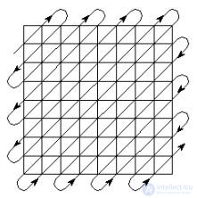
Fig. 15.4
This procedure is called zigzag scanning .
As a result of this transformation, the square matrix of 8x8 quantized DCT coefficients will turn into a linear sequence of 64 numbers, most of which are consecutive zeros. It is known that such streams can be very efficiently compressed by encoding repetition lengths. That is how it is done.
At the next, fifth stage of JPEG- encoding, the resulting chains of zeros are subjected to encoding of repetition lengths.
Finally, the last stage of the JPEG algorithm is the coding of the resulting sequence by some statistical algorithm or algorithms from the LZW series. Usually, Shannon-Fano coding or Huffman algorithm is used. As a result, a new sequence is obtained, the size of which is substantially less than the size of the array of initial data.
The last two stages of coding are usually called secondary compression, and it is here that the statistical lossless coding takes place, and taking into account the characteristic data structure, a significant reduction in their volume.
Decoding data compressed according to the JPEG algorithm is performed in the same way as encoding, but all operations follow in reverse order.
After unpacking using the Huffman method (or LZW) and arranging the linear sequence into blocks of 8x8 in size, the spectral components are dequantized using quantization tables stored during coding. To do this, the unpacked 64 DCT values are multiplied by the corresponding numbers from the table. After that, each block undergoes an inverse cosine transform, the procedure of which coincides with the direct one and differs only in the characters in the transformation matrix. The sequence of actions for decoding and the result obtained are illustrated in the table below. 16.3.
Table 15.3
|
Quantized data | |||||||
15 | 0 | -one | 0 | 0 | 0 | 0 | 0 |
-2 | -one | 0 | 0 | 0 | 0 | 0 | 0 |
-one | -one | 0 | 0 | 0 | 0 | 0 | 0 |
0 | 0 | 0 | 0 | 0 | 0 | 0 | 0 |
0 | 0 | 0 | 0 | 0 | 0 | 0 | 0 |
0 | 0 | 0 | 0 | 0 | 0 | 0 | 0 |
0 | 0 | 0 | 0 | 0 | 0 | 0 | 0 |
0 | 0 | 0 | 0 | 0 | 0 | 0 | 0 |
Dequantized data | |||||||
240 | 0 | -ten | 0 | 0 | 0 | 0 | 0 |
-24 | -12 | 0 | 0 | 0 | 0 | 0 | 0 |
-14 | -13 | 0 | 0 | 0 | 0 | 0 | 0 |
0 | 0 | 0 | 0 | 0 | 0 | 0 | 0 |
0 | 0 | 0 | 0 | 0 | 0 | 0 | 0 |
0 | 0 | 0 | 0 | 0 | 0 | 0 | 0 |
0 | 0 | 0 | 0 | 0 | 0 | 0 | 0 |
0 | 0 | 0 | 0 | 0 | 0 | 0 | 0 |
DCT reverse result | |||||||
144 | 146 | 149 | 152 | 154 | 156 | 156 | 156 |
148 | 150 | 152 | 154 | 156 | 156 | 156 | 156 |
155 | 156 | 157 | 158 | 158 | 157 | 156 | 155 |
160 | 161 | 161 | 162 | 161 | 159 | 157 | 155 |
163 | 163 | 164 | 163 | 162 | 160 | 158 | 156 |
163 | 164 | 164 | 164 | 162 | 160 | 158 | 157 |
160 | 161 | 162 | 162 | 162 | 161 | 159 | 158 |
158 | 159 | 161 | 161 | 162 | 161 | 159 | 158 |
For comparison, the source data | |||||||
139 | 144 | 149 | 153 | 155 | 155 | 155 | 155 |
144 | 151 | 153 | 156 | 159 | 156 | 156 | 156 |
150 | 155 | 160 | 163 | 158 | 156 | 156 | 156 |
159 | 161 | 161 | 160 | 160 | 159 | 159 | 159 |
159 | 160 | 161 | 162 | 162 | 155 | 155 | 155 |
161 | 161 | 161 | 161 | 160 | 157 | 157 | 157 |
161 | 162 | 161 | 163 | 162 | 157 | 157 | 157 |
162 | 162 | 161 | 161 | 163 | 158 | 158 | 15 |
Obviously, the recovered data is slightly different from the original. This is natural because JPEG was designed as a lossy compression.
In the figure below. 15.5 shows the original image (left), as well as an image compressed using the JPEG algorithm 10 times (in the center) and 45 times (right). The loss of quality in the latter case is quite noticeable, but the gain in volume is also obvious.
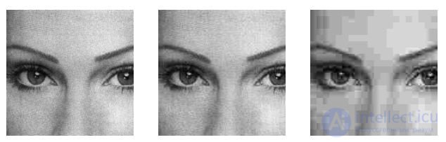
Fig. 15.5
So JPEG compression consists of the following steps:
one. Image splitting into blocks of 8x8 pixels.
2 Apply discrete cosine transform to each block.
3 Rounding DCT coefficients in accordance with a given weight matrix.
four. Convert the matrix of rounded DCT coefficients to a linear sequence by zigzagging them.
five. Repeat coding to reduce the number of zero components.
6 Statistical coding of the result by a Huffman code or arithmetic code.
Decoding is done in the same way, but in reverse order.
Significant positives of the JPEG compression algorithm are:
-the ability to set in a wide range (from 2 to 200) the degree of compression;
-the ability to work with images of any bit depth;
-symmetric compression procedures - unpacking.
The disadvantages include the presence of a halo on sharp color transitions - the Gibbs effect, as well as the disintegration of the image into separate 8x8 squares with a high degree of compression.
15 4 Test questions .
1. Name the types of source information that can be encoded with losses.
2. Why are pre-conversion (DFT) information done in lossy coding methods?
3. What are the main stages of JPEG encoding of images?
4. Why is the matrix 8X8 pixels of the image chosen as the basic element of compression by the JPEG method?
5. What should be the quantization matrix in the JPEG method, if we do not want to lose information in the image?

Comments
To leave a comment
Information and Coding Theory
Terms: Information and Coding Theory