Content
Introduction
Split the original sequence by thinning time
Merge procedure. Count "Butterfly"
Graph FFT algorithm with thinning by time. Binary inverse permutation
Turn factors
Computational efficiency of time thinning FFT algorithm
findings
Introduction
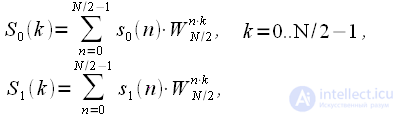
Earlier, expressions were given for the DFT and the scheme of the split-join procedure. We will need them for further presentation, so we will give them without explanation.
The expression for the DFT is:
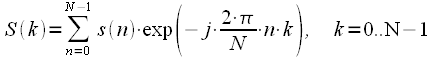 | (one) |
The split-join procedure is shown in Figure 1.
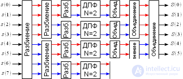
Figure 1: Splitting and combining sequences with N = 8
Split the original sequence by thinning time
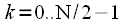
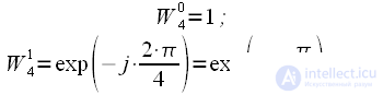
To begin with, the complex exponent in expression (1) is denoted as:
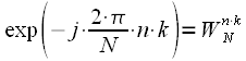 | (2) |
Then the expression (1) takes the form:
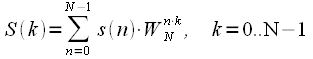 | (3) |
Thinning time consists in splitting the original sequence of samples

,
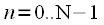
in two sequences of duration


and

,
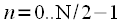
such that
, but
,
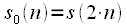
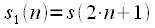
. In other words, the sequence
contains sequence counts
with even indices, and
- with odd ones. Thinning time for N = 8 is clearly shown in Figure 2.

Figure 2: Thinning time for N = 8
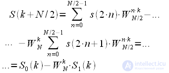
Consider the DFT signal thinned by time:
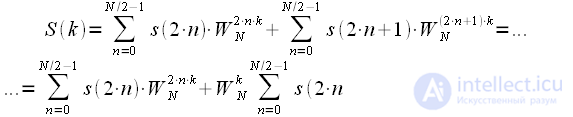 | (four) |
If we consider only the first half of the spectrum

,
and also consider that
 , , | (five) |
then (4) can be written:
 | (6) |
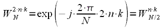
Where

and

,
-
dotted DFT sequences of “even”
and "odd"
,
:
 | (7) |
And what did we get? Thinning in time can be considered an algorithm for splitting a sequence into two half-lengths. The first half of the combined spectrum is the sum of the spectrum of the “even” sequence and the spectrum of the “odd” sequence multiplied by the coefficients

which are called rotational coefficients.
Merge procedure. Count "Butterfly"
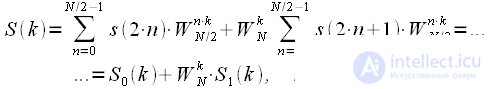
Now consider the second half of the spectrum
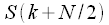
,
:
 | (eight) |
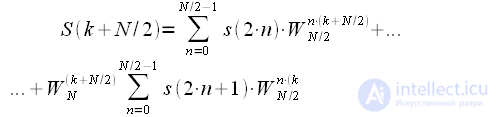
Consider the multiplier in more detail.
 . . | (9) |
Consider that
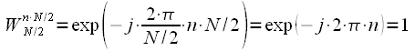 , , | (ten) |
then expression (10) is true for any integer

, then (9) can be written taking into account (10):
 . . | (eleven) |
Consider now the turning factor in (8):
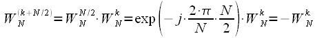 . . | (12) |
Then the expression (8) in view of (11) and (12) takes the form:
 | (13) |
Thus, we can finally write down:
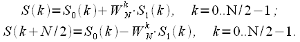 | (14) |
Expression (14) is a combination algorithm for thinning by time. This merging procedure can be represented as a graph (Figure 3), which is called “Butterfly”.
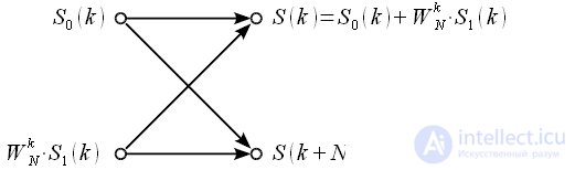
Figure 3: Combining procedure based on the “Butterfly” graph
Graph FFT algorithm with thinning by time. Binary inverse permutation
We represent in the form of a graph an FFT algorithm with decimation in time based on a partitioning - a combination with

(picture 1).
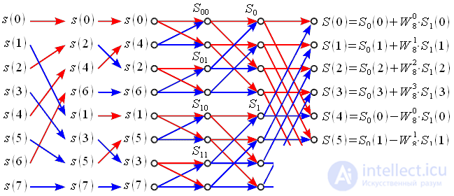
Figure 4: Graph of the FFT algorithm with thinning by time with N = 8
At the first stage, the input signal samples are interchanged and the initial sequence is divided into “even” and “odd sequences” (indicated by red and blue arrows). Then the “even” and “odd” sequences are in turn divided into “even” and “odd” sequences. With

such a division can be done

time. In our case

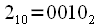
. This procedure is called binary-inverse permutation, so you can renumber the samples by rewriting the reference number in the binary system in the opposite direction. for example

has an index in decimal

, if

rewrite from right to left then we get

, i.e
after splitting into even odd before the first operation "Butterfly" will be in place

which in turn will fall into place
. By a similar rule, all counts will be swapped, while some will remain in place, in particular

as if

rewrite right to left it will still

similarly


and

. It is very important to understand that this renumbering method should be used when writing a number in a binary system consisting of

discharges. In the above example, 3 bits of the binary number were used, but if

(

) then it is necessary to write the number when using 4 digits. In this case
and after rewriting we get

that is, when
will not remain in place but will be swapped with
.
It can be said that directly binary-inverse permutation is convenient when the number of samples of the input signal is fixed in advance, however, in universal algorithms of FFT for various sizes

, binary inverse permutation is not effective, it is easier and faster to swap samples.
After a binary-inverse permutation, we obtain four 2-point DFTs:
 | (15) |
Based on four 2-point DFTs, two 4-point DFTs are formed:
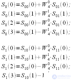 | (sixteen) |
And at the last level the full spectrum of the input signal is formed.
Turn factors
Consider in more detail the turning factors
.
At the first level (expression (15)), only one rotation coefficient is required.

This means that at the first level of the calculation of the spectrum, multiplication operations are not required (multiplication by

are called trivial, since when multiplied by
the multiplier remains the same or changes its sign to the opposite).
At the second level, we have two turning factors:
 | (17) |
Multiplication by an imaginary unit can also be considered trivial, since the real and imaginary parts of a complex number simply change places and change their sign.
At the third level, we already have 4 turning factors:
 | (18) |
Graphically, the steering factors can be represented as vectors on the complex plane:
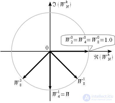
Figure 5: The rotational coefficients of the FFT algorithm with decimation time at N = 8
It can be noted that at all levels of unification the number of pivot coefficients doubles, with all the pivot coefficients of the previous level of unification being present at the next level. Thus, in order to move to the next level, it is necessary to insert the next factors between the rotation coefficients of the current level. Graphically, to go to the next level with N = 16, you need to supplement Figure 5 as shown in Figure 6. Gray vectors show the turning factors that will be present at the last level when
which are not with
.
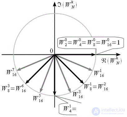
Figure 6: The rotational coefficients of the FFT algorithm with decimation in time at N = 16
It should also be noted that all rotational factors with the exception of zero

are in the lower half-plane of the complex plane.
Computational efficiency of time thinning FFT algorithm
The time thinning algorithm at each level requires
complex multiplications and additions. With
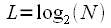
the number of levels of decomposition - the union is
so the total number of multiply and add operations is

.
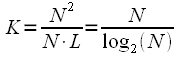
Consider how many times the FFT algorithm with thinning in time is more efficient than the DFT. To do this, consider the acceleration factor

the ratio of the number of complex multiplication and additions using DFT and FFT, while taking into account that
:
 time. time. | (nineteen) |
The table below shows the required number of operations.

for the DFT algorithm for different
and when using FFT with thinning on time.
| four | 6 | eight | ten | 12 |
| sixteen | 64 | 256 | 1024 | 4096 |
| DFT | 256 | 4096 | 65536 | 1048576 | 16777216 |
| FFT | 64 | 384 | 2048 | 10240 | 49152 |
| time | four | 10.7 | 32 | 102.4 | 341 |
The table clearly shows that the use of FFT leads to a significant reduction in the required number of computational operations. So for example when

FFT requires 100 times fewer operations than DFT, and with

341 times! The first publication of these results had the effect of a bombshell, rocking the entire scientific community. At the same time, it is very important that the gain in performance is the greater, the larger the sample size
. So for example when

the gain will be
time.
findings
Thus, in order to obtain an effective FFT algorithm for a base 2 with decimation time, with
it is necessary:
Carry out the binary-inverse permutation of the samples of the input signal, thereby ensuring the splitting of the sequence.
Using the turn factors, make N / 2 operations “Butterfly” according to expression (14) to get the first combination
Repeat the “Butterfly” operation according to expression (14) to merge to the next level
times, also using turning factors.
At the output, we obtain the DFT of the input sequence.

Comments
To leave a comment
Digital signal processing
Terms: Digital signal processing