Content
Introduction
FFT algorithm with decimation in frequency
Algorithm with decimation by frequency
Comparison of base-2 FFT algorithms with decimation in time and frequency
findings
Introduction
Previously, a time-thinned FFT algorithm was considered. In this section, we consider another method of splitting and combining, which is called decimation by frequency.
FFT algorithm with decimation in frequency
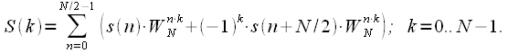
Again, write the expression for the discrete Fourier transform of the signal

:
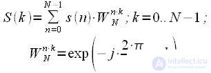 | (one) |
In the FFT algorithm with decimation by time, the original signal was split according to the binary-inverse permutation. And received the first and second half of the spectrum. In the thinning algorithm, on the contrary, the original signal
divided in half, i.e.
and

. Then expression (1) can be rewritten:
 | (2) |
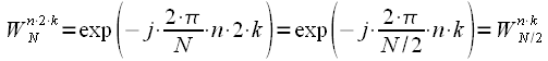
Consider that
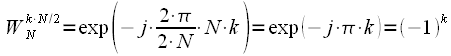 | (3) |
Then
 | (four) |
Let us now consider even spectrum readings.

 | (five) |
Consider that
 | (6) |
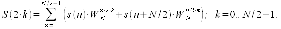
Then
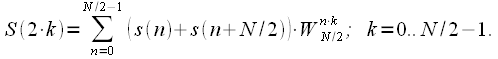 | (7) |
Thus, even spectrum samples are calculated as the DFT of the sum of the first and second half of the original signal.
Now consider the odd spectrum readings.

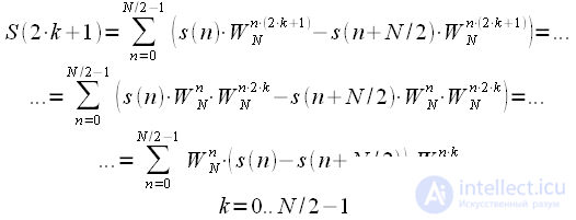 | (eight) |
The final expression for even and odd spectrum reads:
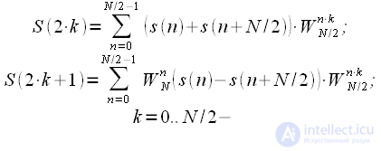 | (9) |
Let us comment on the result obtained based on all the above and with an eye to the decimation algorithm. When dividing the signal into even and odd samples, the first and second halves of the spectrum were obtained in the decimation algorithm. In this case, the algorithm with decimation by frequency, on the contrary, by the first and second half of the signal, allows to calculate even and odd spectral samples (therefore, it is called frequency decay). The difference between the algorithms is that when thinning in time, the multiplication by the rotational coefficients was made after the DFT of an even and odd sequence, and in this algorithm, the multiplication by the rotational coefficients is made before the DFT.
Algorithm with decimation by frequency
The butterfly graph for the thinning algorithm is shown in the figure:
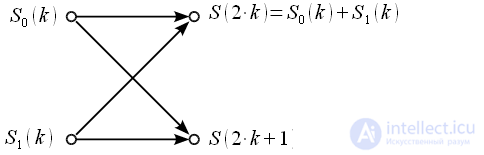
Figure 1: Butterfly graph for frequency decimation FFT algorithm
The pivot coefficients in the decimation frequency algorithm completely coincide with the pivot coefficients of the FFT algorithm with decimation in time.
We represent in the form of a graph an FFT algorithm with decimation in frequency based on a partitioning - a combination with

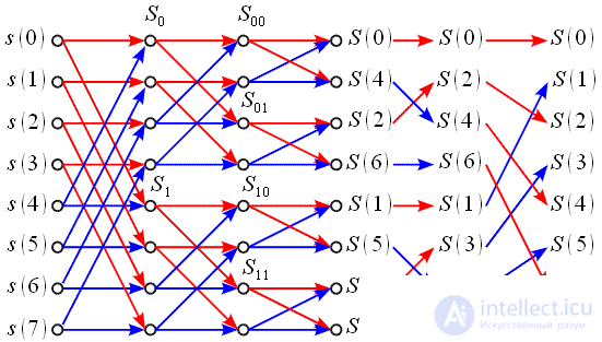
Figure 2: Graph FFT decimation by frequency for N = 8
At the first stage, the initial signal is divided into 2 halves (red and blue arrows). Further calculated
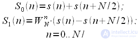 | (ten) |
Then if you do the DFT

, then we obtain even samples of the spectrum in accordance with (9), and if the DFT

- then odd spectrum readings. Thus, one DFT duration
replaced by two DFT duration

. To calculate each of the DFT of half the duration, thinning is again applicable in frequency. As a result, we get:
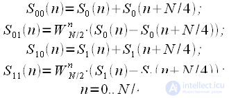 | (eleven) |
As a result, 4 DFTs of 2 points each were obtained, which can also be performed using the butterfly graph. At the output we obtain spectral readings that will be rearranged. At the first level of the transformation, even and odd spectrum samples were obtained; at the second level, even and odd samples were again divided into even and odd ones. As a result, a binary inverse permutation must be applied to place spectral samples in place.
Comparison of base-2 FFT algorithms with decimation in time and frequency
Thus, it is possible to compare the FFT algorithm with decimation in frequency with the FFT algorithm with decimation in time:
1. Binary inverse permutation is used in both algorithms. In the thinning algorithm it is used at the beginning, in the thinning algorithm it is used at the end.
2. In both algorithms, the same rotational coefficients are used. In the time thinning algorithm, the rotational coefficients are multiplied by the result of the shortened DFT, and in the frequency thinning algorithm, the multiplication by the rotational coefficients is carried out to the shortened DFT.
3. In connection with the foregoing, the computational efficiency of both algorithms is almost identical.
findings
Summarize. In a cycle of three articles, ways to reduce computational costs when using the DFT were considered. The most common FFT algorithms with thinning in time and frequency are considered and the effectiveness of these algorithms is shown.
It should be noted that the FFT algorithms are not limited to the decimation algorithm in time and frequency. There are many other algorithms, for example, base four algorithms, generalized algorithms for arbitrary lengths, etc. There is also a grape algorithm that provides the minimum number of multiplications of all possible algorithms. But in practice, the algorithms for base two are the most widely used. This is due to several reasons:
1. Simplicity of software implementation of algorithms and at the same time high efficiency.
2. The winnings obtained by alternative FFT algorithms are insignificant compared to base two algorithms and leveled by exponentially growing processing power of the processors.
3. Algorithms on the base two perfectly "parallelize" when using rigid logic.
All this translates alternative FFT algorithms into the category of “exotic”, and in practice, as a rule, base 2 algorithms are the best choice. However, if the need arises, you can always refer to the literature.
It remains for us to answer the last question: does the FFT algorithm have flaws? It turns out there is. As a result of the fact that the acceleration of calculations is achieved due to the maximum use of the data calculated at the previous stage, the coherent accumulation of rounding errors in the FFT algorithm results in multiplication and addition. However, this effect has a significant effect on fixed-point arithmetic and the representation of numbers with less than 8 digits. When representing floating-point numbers or 8 or higher digits, this effect can be neglected, since it will have almost no effect on the accuracy of the spectrum calculation.

Comments
To leave a comment
Digital signal processing
Terms: Digital signal processing