Lecture
A quantum computer is a computing device that uses the phenomena of quantum superposition and quantum entanglement to transmit and process data. Although the emergence of transistors, classical computers and many other electronic devices is associated with the development of quantum mechanics and condensed matter physics, information between the elements of such systems is usually transmitted in the form of electrical voltage.
A full-fledged quantum computer is still a hypothetical device, the very possibility of constructing which is associated with the serious development of quantum theory in the field of many particles and complex experiments; this work lies at the forefront of modern physics.
The first practical high-level programming language for this type of computer is Quipper, which is based on Haskell [1] .
The idea of quantum computing was proposed by Yuri Manin in 1980 [2] .
One of the first models of a quantum computer was proposed by Richard Feynman [3] in 1981. Soon Paul Benioff described the theoretical foundations of building such a computer [4] .
Also, the concept of a quantum computer in 1983 was proposed by Stephen Wisner in an article that he had tried to publish for more than ten years before. [5] [6]
The need for a quantum computer arises when we try to investigate complex multi-particle systems, like biological ones, using the methods of physics. The space of quantum states of such systems grows as an exponent of the number  real particles, which makes it impossible to simulate their behavior on classical computers for
  . Therefore, Vizner and Feynman expressed the idea of building a quantum computer.
A quantum computer uses for calculations not ordinary (classical) algorithms, but processes of a quantum nature, so-called quantum algorithms that use quantum-mechanical effects, such as quantum parallelism and quantum entanglement.
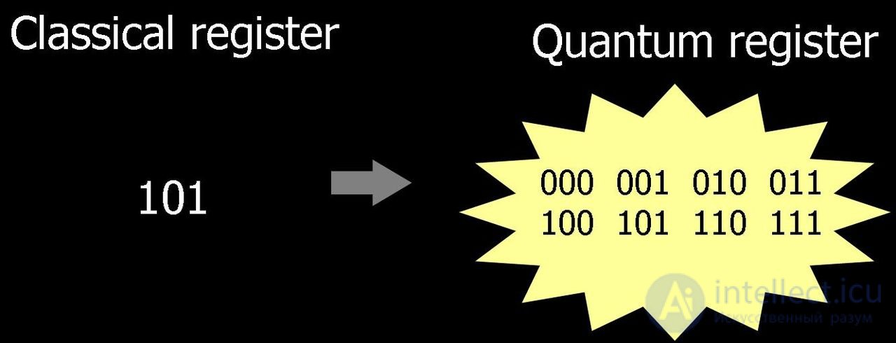
If a classic processor at any moment can be in exactly one of the states 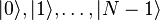 (Dirac designations), then the quantum processor at each moment is simultaneously in all these basic states, with each state
  - with its complex amplitude
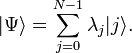
  . This quantum state is called “quantum superposition” of these classical states and is denoted by
Baseline states may also have a more complex form. Then a quantum superposition can be illustrated, for example, as follows: “Imagine an atom that could undergo radioactive decay in a certain period of time. Or do not undergo. We can expect that this atom has only two possible states: “decay” and “not decay”, <...> but in quantum mechanics an atom can have some kind of unified state - “decay - not decay”, that is, nothing else, but between. This state is called “superposition” [7] .
Quantum state  may vary in time in two fundamentally different ways:
If classic states there are spatial positions of a group of electrons in quantum dots controlled by an external field  , then the unitary operation is the solution of the Schrödinger equation for this potential.
Measurement is a random variable taking values  with probabilities
  respectively. This is Born's quantum mechanical rule. Measurement is the only way to obtain information about the quantum state, since the values are not directly accessible to us. The measurement of the quantum state cannot be reduced to the unitary Schrödinger evolution, since, unlike the latter, it is irreversible. During the measurement, the so-called collapse of the wave function occurs. whose physical nature is not completely clear. Spontaneous harmful state measurements during computation lead to decoherence, that is, deviation from unitary evolution, which is the main obstacle in the construction of a quantum computer (see the physical implementations of quantum computers).
A quantum computation is a sequence of unitary operations of a simple form controlled by a classical controlling computer (over one, two, or three qubits). At the end of the calculation, the state of the quantum processor is measured, which gives the desired result of the calculation.
The content of the concept of “quantum parallelism” in the calculation can be disclosed as follows: “The data in the calculation process is quantum information, which, at the end of the process, is transformed into classical information by measuring the final state of the quantum register. The gain in quantum algorithms is achieved due to the fact that when using a single quantum operation, a large number of coefficients of superposition of quantum states, which in the virtual form contain classical information, are transformed at the same time ” [8] .
 |
This section of the article should be wiked.
Please issue it according to the rules for the articles.
|
The idea of quantum computation is that a quantum system of L two-level quantum elements (quantum bits, qubits) has 2 L linearly independent states, and therefore, due to the principle of quantum superposition, the state space of such a quantum register is 2 L -dimensional Hilbert space. The operation in quantum computations corresponds to the rotation of the register state vector in this space. Thus, a quantum computing device of the size L qubit actually uses simultaneously 2 L classical states.
The physical systems that implement qubits can be any objects that have two quantum states: polarization states of photons, electronic states of isolated atoms or ions, spin states of atomic nuclei, etc.
One classic bit can be in one and only one of the states  or
or  . A quantum bit, called a qubit, is in a state
 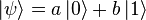 so | a | ² and | b | ² - the probability to get 0 or 1, respectively, when measuring this state;
  ; | a | ² + | b | ² = 1. Immediately after the measurement, the qubit enters the basic quantum state corresponding to the classical result.
Example:
There is a qubit in the quantum state 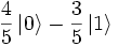
In this case, the probability to get when measuring
| 0 | makes up | (4/5) ² = 16/25 | = 0.64, |
| one | (-3/5) ² = 9/25 | = 0.36. |
In this case, when measuring, we got 0 with a 0.64 probability.
As a result of measurement, the qubit enters a new quantum state. , that is, by the next measurement of this qubit we get 0 with one hundred percent probability (it is assumed that by default the unitary operation is identical; in real systems this is not always the case).
Let us explain for explanation two examples from quantum mechanics: 1) the photon is in the state  superposition of two polarizations. This state is a vector in a two-dimensional plane, the coordinate system in which can be represented as two perpendicular axes, so
  and
and  there are projections on these axes; measurement once and for all collapses the state of the photon into one of the states or and the probability of collapse is equal to the square of the corresponding projection. The total probability is obtained by the Pythagorean theorem.
Let us turn to a system of two qubits. The measurement of each of them can give 0 or 1. Therefore, the system has 4 classical states: 00, 01, 10 and 11. Similar to them the basic quantum states:  . Finally, the total quantum state of the system is
  . Now | a | ² is the probability to measure 00, etc. Note that | a | ² + | b | ² + | c | ² + | d | ² = 1 as the total probability.
If we measure only the first qubit of a quantum system in a state , we will succeed:
 first qubit will go to state and the second state
 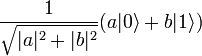 ,
, first qubit will go to state and the second state
  .
.In the first case, the measurement will give the state 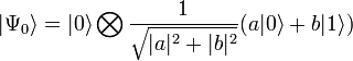 in the second - the state
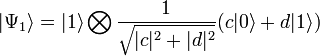
We again see that the result of such a measurement cannot be recorded as a vector in the Hilbert state space. Such a state, in which our ignorance of what kind of result is obtained on the first qubit, is called a mixed state. In our case, this mixed state is called the projection of the original state. on the second qubit, and recorded in the form of a density matrix of the form 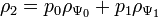 where is density matrix defined as
  .
.
In the general case, a system of L qubits, it has 2 L classical states (00000 ... (L-zeros), ... 00001 (L-digits), ..., 11111 ... (L-ones)), each of which can be measured with probabilities 0—1.
Thus, one operation on a group of qubits is calculated immediately over all its possible values, in contrast to the group of classical bits, when only one current value can be used. This provides unprecedented parallelism of computations.
A simplified calculation scheme on a quantum computer looks like this: a qubit system is taken, on which the initial state is written. Then the state of the system or its subsystems is changed by means of unitary transformations that perform certain logical operations. In the end, the value is measured, and this is the result of the computer. The role of the wires of a classical computer is played by qubits, and the role of logical blocks of a classical computer is played by unitary transformations. This concept of a quantum processor and quantum logic gates was proposed in 1989 by David Deutsch. David Deutsch also found a universal logic unit in 1995 with which it is possible to perform any quantum computation.
It turns out that two basic operations are enough to build any calculation. The quantum system gives the result, which is only with some probability the correct one. But at the expense of a small increase in operations in the algorithm, one can arbitrarily approximate the probability of getting the correct result to one.
With the help of basic quantum operations, it is possible to simulate the operation of ordinary logic elements from which ordinary computers are made. Therefore, any problem that is solved now, the quantum computer will solve, and almost the same time. Therefore, the new calculation scheme will be no weaker than the current one.
Most modern computers work in the same way: n bits of memory store a state and each time step is changed by the processor. In the quantum case, a system of n qubits is in a state that is a superposition of all the base states, so the change in the system applies to all 2 n base states at the same time. Theoretically, the new scheme can work much (exponentially) faster than the classical one. In practice, Grover’s (quantum) database search algorithm shows a quadratic increase in power versus classical algorithms.
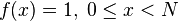 during
  . particles in almost linear time using
  qubit
qubitIt was shown that “quantum acceleration” is not possible for any algorithm. Moreover, the possibility of obtaining quantum acceleration for an arbitrary classical algorithm is a rarity [9] .
One qubit can be represented as an electron in a double-well potential, so that means finding it in the left hole, and - on the right. This is called a qubit on charge states. General view of the quantum state of such an electron:  . Its dependence on time is dependence on time amplitudes.
  ; it is given by the Schrödinger equation
 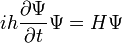 where is the Hamiltonian
  has the same kind of pits and hermitic appearance
 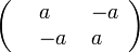 for some constant so the vector
 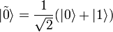 is the eigenvector of this Hamiltonian with an eigenvalue of 0 (the so-called ground state), and
 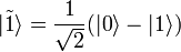 - own vector with value
  (first excited state). There are no other eigenstates (with a certain energy value), since our problem is two-dimensional. As each state goes over time
  in state
  , then to implement the NOT operation (transition
  and vice versa, just wait for a moment
  . That is, the NOT gate is given simply by the natural quantum evolution of our qubit, provided that the external potential defines a two-well structure; This is done using quantum dot technology.
To implement a CNOT, two qubits (that is, two pairs of holes) must be arranged perpendicular to each other, and in each of them should be arranged in a separate electron. Then constant for the first (controlled) pair of holes it will depend on the state of the electron in the second (controlling) pair of holes: if closer to the first, will be more, if further - less. Therefore, the state of the electron in the second pair determines the time of the NOT in the first well, which allows you to select the desired length of time again for the production of the CNOT operation.
This scheme is very approximate and idealized; real schemes are more complicated and their implementation presents a challenge to experimental physics.
Teleportation allows you to transfer the quantum state of the system using conventional classical communication channels. Thus, it is possible, in particular, to obtain the bound state of a system consisting of subsystems remote for a long distance.
The main problems associated with the creation and use of quantum computers:
Благодаря огромной скорости разложения на простые множители, квантовый компьютер позволит расшифровывать сообщения, зашифрованные асимметричным криптографическим алгоритмом RSA. До сих пор этот алгоритм считается сравнительно надёжным, так как эффективный способ разложения чисел на простые множители для классического компьютера в настоящее время неизвестен. Для того, например, чтобы получить доступ к кредитной карте, нужно разложить на два простых множителя число длиной в сотни цифр. Даже для самых быстрых современных компьютеров выполнение этой задачи заняло бы в сотни раз больше времени, чем возраст Вселенной. Благодаря алгоритму Шора эта задача становится вполне осуществимой, если квантовый компьютер будет построен.
Применение идей квантовой механики уже открыли новую эпоху в области криптографии, так как методы квантовой криптографии открывают новые возможности в области передачи сообщений [10] . Прототипы систем подобного рода находятся на стадии разработки [11] .
Построение квантового компьютера в виде реального физического прибора является фундаментальной задачей физики XXI века. По состоянию на начало 2010-х годов построены только ограниченные его варианты (самые большие сконструированные квантовые регистры имеют немногим более десятка связанных кубит [12] [13] ). Вопрос о том, до какой степени возможно масштабирование такого устройства (так называемая «Проблема масштабирования»), является предметом новой интенсивно развивающейся области — многочастичной квантовой механики . Центральным здесь является вопрос о природе декогерентности (точнее, о коллапсе волновой функции), который пока остаётся открытым. Различные трактовки этого процесса можно найти в книгах [14] [15] [16] .
Главные технологии для квантового компьютера:
На рубеже XXI века во многих научных лабораториях были созданы однокубитные квантовые процессоры (по существу, управляемые двухуровневые системы, о которых можно было предполагать возможность масштабирования на много кубитов).
В конце 2001 года IBM заявила об успешном тестировании 7-кубитного квантового компьютера, реализованного с помощью ЯМР. На нём был исполнен алгоритм Шора и были найдены сомножители числа 15 [17] .
В 2005 году группой Ю. Пашкина (кандидат физ.-мат. наук, старший научный сотрудник лаборатории сверхпроводимости г. Москвы) при помощи японских специалистов был построен двухкубитный квантовый процессор на сверхпроводящих элементах [18] .
В ноябре 2009 года физикам из Национального института стандартов и технологий в США впервые удалось собрать программируемый квантовый компьютер, состоящий из двух кубит [19] .
В феврале 2012 года компания IBM сообщила о достижении значительного прогресса в физической реализации квантовых вычислений с использованием сверхпроводящих кубитов, которые, по мнению компании, позволят начать работы по созданию квантового компьютера [20] .
В апреле 2012 года группе исследователей из Южно-Калифорнийского университета, Технологического университета Дельфта, университета штата Айова, иКалифорнийского университета, Санта-Барбара, удалось построить двухкубитный квантовый компьютер на кристалле алмаза с примесями. Компьютер функционирует при комнатной температуре и теоретически является масштабируемым. В качестве двух логических кубитов использовались направления спина электрона и ядра азота соответственно. Для обеспечения защиты от влияния декогерентности была разработана целая система, которая формировала импульс микроволнового излучения определённой длительности и формы. При помощи этого компьютера реализован алгоритм Гровера для четырёх вариантов перебора, что позволило получить правильный ответ с первой попытки в 95 % случаев [21] [22] .
Канадская компания D-Wave Systems (англ.)русск. с 2007 года заявляла о создании различных вариантов квантового компьютера: 16 кубит - Orion [23] [24] , 28 кубит в ноябре 2007 [25] , D-Wave One (англ.)русск. с 128-кубитным чипом в мае 2011 [26] , процессор Vesuvius на 512 кубитов в конце 2012 года [27] , более 1000 кубит в июне 2015 [28] . Компания получала инвестиции из множества источников, например 17 млн долларов США в январе 2008 года [29] , также проводилисьраспределённые вычисления AQUA@home ( A diabatic QU antum A lgorithms) [30] для тестирования алгоритмов оптимизации для адиабатических сверхпроводящих квантовых компьютеров D-Wave .
Компьютеры D-Wave работают на принципе квантовой релаксации (квантовый отжиг), могут решать крайне ограниченный подкласс задач оптимизации, и не подходят для реализации традиционных квантовых алгоритмов и квантовых вентилей [31] (Quantum Annealing [32] ).
D-Wave демонстрировала решение на своих компьютерах некоторых задач, например, распознавания образов (8 декабря 2009 года на конференцииNIPS ( англ. ) при участии Hartmut Neven ( англ. ) [33] , исследования трехмерной формы белка по известной последовательности аминокислот (август 2012) [34] .
The operating temperature of superconducting chips in D-Wave devices is about 20 μK, there is careful shielding from external electric and magnetic fields [35] [36] .
Since May 20, 2011, D-Wave Systems has been selling the D-Wave One quantum computer (128 qubits) for $ 11 million, which solves only one problem — discrete optimization [37] . Among the customers of D-Wave is Lockheed Martin (since May 2011), the contract concerns the performance of complex calculations on quantum processors and includes the maintenance of the D-Wave One quantum computer [38] .
At the same time, D-Wave Systems quantum computers are criticized by some researchers. So, associate professor of the Massachusetts Institute of Technology Scott Aaronson believes that D-Wave has not yet been able to prove that its computer solves any problems faster than a regular computer, or that the 128 qubits used can be entered in quantum entanglement. If qubits are not in a tangled state, then this is not a quantum computer [39] .
In May 2013, Amherst College professor from the Canadian province of Nova Scotia, Catherine McGeoch, announced her comparison of the D-Wave One computer on a Vesuvius processor with a traditional computer with an Intel microprocessor. In the first test, one of the tasks of the QUBO class, which is well suited to the structure of the processor, was performed by D-Wave One in 0.5 seconds, while the computer with an Intel processor took 30 minutes (3600 times). In the second test, a special program was needed to “translate” the task into the language of the D-Wave computer and the computation speed of the two computers was approximately equal. In the third test, which also required a “translation” program, the D-Wave One computer in 30 minutes found a solution to 28 of 33 set tasks, while a computer on an Intel processor found a solution for only 9 problems [40] .
In January 2014, D-Wave scientists published an article stating that using the qubit tunnel spectroscopy method [41] they proved the presence of quantum coherence and entanglement between separate subgroups of qubits (2 and 8 elements) in the processor during calculations [42] .
продолжение следует...
Часть 1 Quantum computer

Comments
To leave a comment
Quantum informatics
Terms: Quantum informatics