Lecture
Numerical methods for solving the Cauchy problem for first-order ODU
Numerical methods for solving first-order ODE systems
The finite difference method for solving boundary value problems for ODE
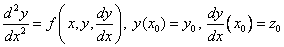
Many problems of science and technology are reduced to the solution of ordinary differential equations (ODE). ODE are called such equations that contain one or more derivatives of the desired function. In general, the ODE can be written as follows:
 where x is an independent variable
  - i-th derivative of the desired function. n is the order of the equation. The general solution of the nth order ODE contains n arbitrary constants
  i.e. the general solution is
  .
.
To select a single solution, you must specify n additional conditions. Depending on how additional conditions are specified, there are two different types of tasks: the Cauchy problem and the boundary value problem. If the additional conditions are set at one point, then this problem is called the Cauchy problem. The additional conditions in the Cauchy problem are called initial conditions. If additional conditions are specified at more than one point, i.e. for different values of the independent variable, then this problem is called the boundary value. The additional conditions themselves are called boundary or boundary conditions.
It is clear that for n = 1 we can speak only about the Cauchy problem.
Examples of the formulation of the Cauchy problem :

Examples of boundary value problems :

Such problems can be solved analytically only for some special types of equations.
Task setting . Find a solution to the first order ODE
 on the segment
  provided
When finding an approximate solution, we will assume that the calculations are carried out with a calculated step  , the calculated nodes are points
  spacing [ x 0 , x n ].
The goal is to build a table.
x i | x 0 | x 1 | ... | x n |
y i | y 0 | y 1 | ... | y n |
those. look for approximate values of y in the grid nodes.
Integrating the equation on the segment  get
get
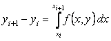
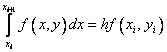
A completely natural (but not unique) way to obtain a numerical solution is to replace the integral in it with some quadrature numerical integration formula. If we use the simplest formula of left rectangles of the first order
 ,
,
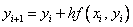
then we obtain the explicit Euler formula :
 ,
,  .
.
Payment procedure:
Knowing  find
find 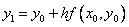 then
then 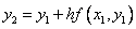 etc.
etc.
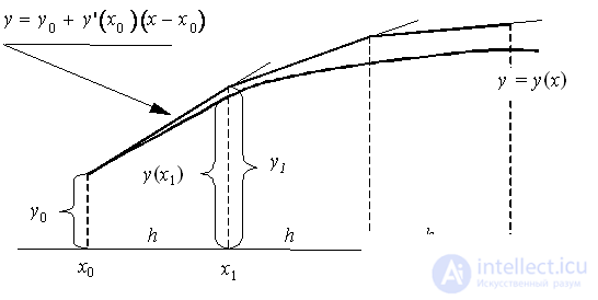
Geometric interpretation of the Euler method :
Using the fact that at the point x 0 we know the solution y ( x 0 ) = y 0 and the value of its derivative 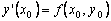 , you can write the equation of the tangent to the graph of the desired function
  at the point
  :
: 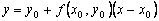 . With a sufficiently small step h the ordinate
 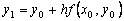 this tangent, obtained by substituting in the right side of the value
  , should differ little from the ordinate y ( x 1 ) of the solution y ( x ) of the Cauchy problem. Hence the point
  the intersection of the tangent with the line x = x 1 can be approximately taken as a new starting point. Through this point we will again draw a straight line.
 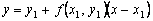 which approximately reflects the behavior of the tangent to at the point
  . Substituting here
  (i.e. the intersection with the line x = x 2 ), we obtain an approximate value of y ( x ) at the point x 2 :
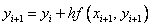
 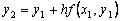 etc. As a result, for the i –th point we obtain the Euler formula.
The explicit Euler method has the first order of accuracy or approximation.
If you use the formula of the right rectangles:  then we come to the method
 , .
, .
This method is called the implicit Euler method , because to calculate the unknown value  by known value
  it is required to solve an equation, generally non-linear.
The implicit Euler method has the first order of accuracy or approximation.
Modified Euler method: in this method, the calculation  consists of two stages:
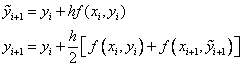
This scheme is also called the predictor - corrector method (predicting - correcting). At the first stage, the approximate value is predicted with low accuracy (h), and at the second stage this prediction is corrected, so that the resulting value has a second order of accuracy.
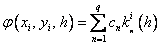
Runge – Kutta methods: the idea of constructing explicit Runge – Kutta methods of the p –th order is to obtain approximations to the values of y ( x i +1 ) using the formula
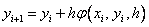 ,
,
Where

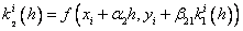
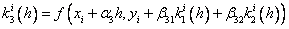
…………………………………………….
 .
.
Here a n , b nj , p n ,  - some fixed numbers (parameters).
When building the Runge – Kutta methods, the parameters of the function  ( a n , b nj , p n ) is chosen in such a way as to obtain the desired order of approximation.
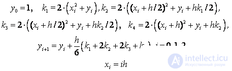
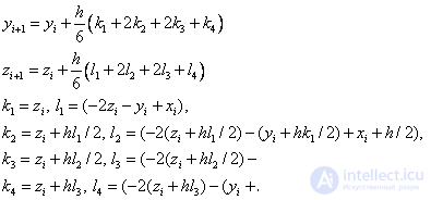
Runge - Kutta fourth order accuracy scheme :

An example . Solve the Cauchy problem:
 .
.
Consider three methods: the explicit Euler method, the modified Euler method, the Runge - Kutta method.
Exact solution: 
The calculated formulas for the explicit Euler method for this example:

The design formulas of the modified Euler method:

Calculation formulas of the Runge – Kutta method:
x | y1 | y2 | y3 | exact |
0 | 1.0000 | 1.0000 | 1.0000 | 1.0000 |
0.1 | 1.2000 | 1.2210 | 1.2221 | 1.2221 |
0.2 | 1.4420 | 1.4923 | 1.4977 | 1.4977 |
0.3 | 1.7384 | 1.8284 | 1.8432 | 1.8432 |
0.4 | 2.1041 | 2.2466 | 2.2783 | 2.2783 |
0.5 | 2.5569 | 2.7680 | 2.8274 | 2.8274 |
0.6 | 3.1183 | 3.4176 | 3.5201 | 3.5202 |
0.7 | 3.8139 | 4.2257 | 4.3927 | 4.3928 |
0.8 | 4.6747 | 5.2288 | 5.4894 | 5.4895 |
0.9 | 5.7377 | 6.4704 | 6.8643 | 6.8645 |
one | 7.0472 | 8.0032 | 8.5834 | 8.5836 |
y1 is the Euler method, y2 is the modified Euler method, y3 is the Runge Kutt method.
It can be seen that the most accurate is the Runge – Kutta method.
The considered methods can also be used to solve systems of differential equations of the first order.
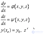
We show this for the case of a system of two first order equations:
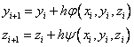
Explicit Euler Method:
Modified Euler method:

Runge - Kutta fourth order accuracy scheme:

The Cauchy problem for equations of higher order are also reduced to solving systems of equations of ODE. For example, consider the Cauchy problem for a second order equation
We introduce the second unknown function  . Then the Cauchy problem is replaced by the following:

Those. in terms of the previous problem: 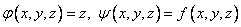 .
.
Example. Find a solution to the Cauchy problem :
 on the interval [0,1].
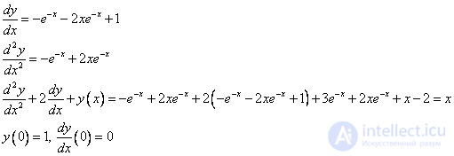
Exact solution: 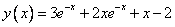
Really:
We solve the problem by the explicit Euler method, modified by the Euler and Runge-Kutt method with a step h = 0.2.
We introduce a function  .
.
Then we obtain the following Cauchy problem for a system of two ODUs of the first order:

Explicit Euler Method:

Modified Euler method:

Runge – Kutta method:
Euler scheme:
X | y | z | y theor | z theor | yy theor |
0 | one | 0 | one | 0 | 0 |
0.2 | one | -0.2 | 0.983685 | -0.14622 | 0.016315 |
0.4 | 0.96 | -0.28 | 0.947216 | -0.20658 | 0.012784 |
0.6 | 0.904 | -0.28 | 0.905009 | -0.20739 | 0.001009 |
0.8 | 0.848 | -0.2288 | 0.866913 | -0.16826 | 0.018913 |
one | 0.80224 | -0.14688 | 0.839397 | -0.10364 | 0.037157 |
Modified Euler method:
X | ycv | zcv | y | z | y theor | z theor | yy theor |
0 | one | 0 | one | 0 | one | 0 | 0 |
0.2 | one | -0.2 | one | -0.18 | 0.983685 | -0.14622 | 0.016315 |
0.4 | 0.96 | -0.28 | 0.962 | -0.244 | 0.947216 | -0.20658 | 0.014784 |
0.6 | 0.904 | -0.28 | 0.9096 | -0.2314 | 0.905009 | -0.20739 | 0.004591 |
0.8 | 0.848 | -0.2288 | 0.85846 | -0.17048 | 0.866913 | -0.16826 | 0.008453 |
one | 0.80224 | -0.14688 | 0.818532 | -0.08127 | 0.839397 | -0.10364 | 0.020865 |
Runge - Kutta scheme:
x | Y | z | k1 | l1 | k2 | l2 | k3 | l3 | k4 | l4 |
0 | one | 0 | 0 | -one | -0.1 | -0.7 | -0.07 | -0.75 | -0.15 | -0.486 |
0.2 | 0.983667 | -0.1462 | -0.1462 | -0.49127 | -0.19533 | -0.27839 | -0.17404 | -0.31606 | -0.20941 | -0.13004 |
0.4 | 0.947189 | -0.20654 | -0.20654 | -0.13411 | -0.21995 | 0.013367 | -0.2052 | -0.01479 | -0.2095 | 0.112847 |
0.6 | 0.904977 | -0.20734 | -0.20734 | 0.10971 | -0.19637 | 0.208502 | -0.18649 | 0.187647 | -0.16981 | 0.27195 |
0.8 | 0.866881 | -0.16821 | -0.16821 | 0.269542 | -0.14126 | 0.332455 | -0.13497 | 0.317177 | -0.10478 | 0.369665 |
one | 0.839366 | -0.1036 | -0.1036 | 0.367825 | -0.06681 | 0.40462 | -0.06313 | 0.393583 | -0.02488 | 0.423019 |
Max (yy theor) = 4 * 10 -5
Problem statement : find a solution to a linear differential equation
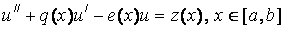 , (one)
satisfying the boundary conditions:  . (2)
. (2)
Theorem. Let be  . Then there is the only solution to the problem.
This problem is reduced, for example, to the problem of determining the deflections of a beam, which is hinged at the ends.
The main stages of the finite difference method:
1) the area of continuous change of the argument ([a, b]) is replaced by a discrete set of points, called nodes:  .
.
2) The desired function of the continuous argument x is approximately replaced by the function of the discrete argument on the given grid, i.e. 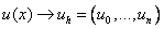 . Function
  called mesh.
3) The original differential equation is replaced by the difference equation for the grid function. Such a replacement is called a differential approximation.
Thus, the solution of the differential equation is reduced to finding the values of the grid function at the grid nodes, which are found by solving algebraic equations.
Approximation of derivatives.
For approximation (replacement) of the first derivative, you can use the formulas:
 - right differential derivative,
 - left differential derivative,
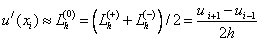 - central differential derivative.
i.e., there are many possible ways to approximate a derivative.
All these definitions follow from the notion of derivative as a limit: 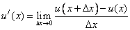 .
.
Based on the difference approximation of the first derivative, it is possible to construct a difference approximation of the second derivative:
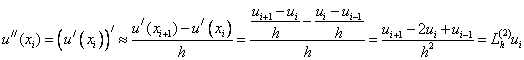 (3)
(3)
Similarly, one can obtain approximations of higher order derivatives.
Definition The approximation error of the nth derivative is the difference: 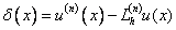 .
.
To determine the order of approximation, a Taylor series expansion is used.
Consider the right difference approximation of the first derivative:

Those. the right difference derivative has the first approximation order in h .
Similarly for the left differential derivative.
The central difference derivative has the second order of approximation .
The approximation of the second derivative by the formula (3) also has the second order of approximation.
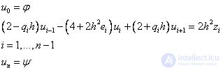
In order to approximate a differential equation, it is necessary to replace in it all the derivatives with their approximations. Consider problem (1), (2) and replace in (1) the derivatives:
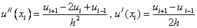 .
.
As a result, we get:
 (four)
The order of approximation of the original problem is 2, since the second and first derivatives are replaced with order 2, and the others are accurate.
So, instead of differential equations (1), (2), a system of linear equations is obtained to determine  in grid nodes.
The scheme can be represented as:
i.e., obtained a system of linear equations with a matrix:

This matrix is three-diagonal, i.e. all elements that are not located on the main diagonal and the two diagonals adjacent to it are equal to zero.
Solving the resulting system of equations, we get the solution to the original problem.
To solve such SLAEs, there is an economical sweep method .
Consider a sweep method for SLAE :
 (one)
(one)
We look for the solution of this system in the form:
 (2)
(2)
Substituting in the first equation, we get:

Here it is taken into account that this ratio should be satisfied for any 
Because
 , (3)
, (3)
then substituting (3) into the second equation, we get:
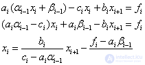
Comparing with (2) we get
 .
.
So you can find all  .
.
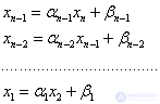
Then from the last equation (1) we find:

Then we consistently find:
Таким образом, алгоритм метода прогонки можно представить в виде:
1) Находим 
2) Для i=1,n-1: (four)
3) Находим 
4) Для i=n-1 до 1 находим: 
Шаги 1),2) – прямой ход метода прогонки, 3),4) – обратный ход метода прогонки.
Теорема . Пусть коэффициенты a i , b i системы уравнений при i =2, 3, …, n–1 отличны от нуля и пусть
 при i =1, 2, 3, …, n. Тогда прогонка корректна и устойчива .
При выполнении этих условий знаменатели в алгоритме метода прогонки не обращаются в нуль и, кроме того, погрешность вычислений, внесенная на каком либо шаге вычислений, не будет возрастать при переходе к следующим шагам. Данное условие есть ни что иное, как условие диагонального преобладания.
Для нашей краевой задачи имеем :

Then: , ,

For our problem, the stability condition is:
 .
.
Let be
 . (6)
. (6)
Then 
Example. Find a solution to the problem:

We write the difference scheme

The condition of stability will become 
Take  .
.
Then 

Or
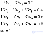
The sweep formulas were obtained for SLAE (1):

Here x is replaced by u.
Consequently,

Solve SLAU sweep method. Calculations arrange in the form of a table:
I | a i | c i | b i | f i | alfa i | beta i | u i |
one | 51 | 35 | 0.2 | 0.6863 | -0.0039 | 0.4701 | |
2 | 15 | 51 | 35 | 0.4 | 0.8598 | -0.0113 | 0.6906 |
3 | 15 | 51 | 35 | 0.6 | 0.9186 | -0.0202 | 0.8164 |
four | 15 | 51 | 35 | 0.8 | 0.9403 | -0.0296 | 0.9107 |
five | 0 | -one | one | 1.0000 |
The procedure for calculating the formulas (4):


The answer is in column u i .
If you forget the formulas, they can be easily derived. The main thing to remember is the basic formula:

Direct move

Reverse

In practice, often boundary conditions can have a more general form.
Рассмотрим следующую краевую задачу :
Найти решение ОДУ 2-го порядка
 ,
,
удовлетворяющую краевым условиям:


В этом случае при построении разностной схемы необходимо еще аппроксимировать и краевые условия.
Аппроксимация:
В результате получим разностную схему:

Or

Мы получили СЛАУ типа (5) с трехдиагональной матрицей, решение которой также можно найти методом прогонки.

Comments
To leave a comment
Numerical methods
Terms: Numerical methods