2. Methods for solving systems of linear algebraic equations

Direct methods for solving SLAE:
Cramer Method
Inverse Matrix Method
Gauss Method
Iterative methods for solving linear algebraic systems:
Simple iteration method or Jacobi method
Gauss-Seidel Method

Numerous practical problems are reduced to solving systems of linear algebraic equations (according to some estimates, more than 75% of all problems). It can be rightly argued that solving linear systems is one of the most common and important tasks in computational mathematics.

Of course, there are many methods and modern software packages for solving SLAEs, but in order to use them successfully, it is necessary to understand the basics of building methods and algorithms, to have an idea of ​​the disadvantages and advantages of the methods used.

Formulation of the problem

It is required to find a solution to the system of m linear equations, which is written in the general form as

,

This system of equations can also be written in matrix form:

,

Where , , .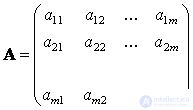

A is the system matrix, - vector of the right parts, - vector of unknowns.

With known A and required to find such , with the substitution of which into the system of equations, it turns into an identity.

A necessary and sufficient condition for the existence of a unique solution of a SLAE is the condition det A ≠ 0, i.e. the determinant of the matrix A is not zero. If the determinant is equal to zero, then the matrix A is called degenerate and, at the same time, the SLAE either does not have a solution or has an infinite number of them.

In the future we will assume the presence of a unique solution.

All methods for solving linear algebraic problems can be divided into two classes: direct (exact) and iterative (approximate).

Direct methods for solving SLAE

Cramer Method

With a small dimension of the system m (m = 2, ..., 5), in practice, Kramer’s formulas are often used to solve the SLAE:

(i = 1, 2, ..., m). These formulas allow one to find the unknowns in the form of fractions whose denominator is the determinant of the system's matrix, and the numerator determines the determinants of the matrices A i obtained from A by replacing the column of coefficients with the free members calculated by the unknown . So A 1 is obtained from the matrix A by replacing the first column with the column of the right sides of f.

For example, for a system of two linear equations

The dimension of the system (i.e., the number m) is the main factor due to which Cramer's formulas cannot be used to numerically solve a high order SLAE. With the direct disclosure of determinants, the solution of a system with m unknowns requires about m! * M arithmetic operations. Thus, to solve a system, for example, from m = 100 equations, 10,158 computational operations will need to be performed (the process will take approximately 10-19 years ), which is beyond the power of even the most powerful modern computer

Inverse Matrix Method

If det A ≠ 0, then there is an inverse matrix . Then the solution of SLAE is written in the form: . Consequently, the solution of the SLAE was reduced to multiplying the known inverse matrix by the vector of the right sides . Thus, the problem of solving a SLAE and the problem of finding an inverse matrix are interconnected; therefore, often the solution of a SLAE is called the task of inverting the matrix. The problems of using this method are the same as when using the Cramer method: finding the inverse matrix is ​​a time consuming operation .

Gauss Method

The most famous and popular direct method for solving SLAEs is the Gauss method . This method consists in the sequential elimination of unknowns. Let in the system of equations

first element . Let's call it the leading element of the first row. Let's divide all the elements of this line by and exclude x 1 from all subsequent lines, starting with the second, by subtracting the first (converted) multiplied by the coefficient at in the appropriate line. Will get

.

If a , then, continuing a similar exception, we arrive at a system of equations with an upper triangular matrix

.

From it in the reverse order we find all the values ​​of x i :

.

The process of bringing to a system with a triangular matrix is ​​called a direct move , and finding the unknowns is called the reverse . If one of the leading elements is zero, the described algorithm of the Gauss method is not applicable. In addition, if any of the leading elements are small, then this leads to increased rounding errors and degraded counting accuracy. Therefore, another variant of the Gauss method is usually used - the Gauss scheme with the choice of the main element . By interchanging the rows as well as the columns with the corresponding renumbering of the coefficients and the unknowns, the condition is satisfied:

, j = i + 1, i + 2, ..., m;

those. The selection of the first main element is made Rearranging the equations so that in the first equation the coefficient a 11 is maximum modulo . Dividing the first line into the main element, as before, exclude x 1 from the remaining equations. Then for the remaining columns and rows select the second main element, etc.

Consider the application of the Gauss method with the choice of the main element on the example of the following system of equations:

In the first equation, the coefficient at = 0, in the second = 1 and in the third = -2, i.e. maximum modulus coefficient in the third equation. Therefore, we rearrange the third and first equation:

Exclude from the second and third equations using the first. In the second equation it is not necessary to exclude. To exclude from the third equation, multiply the first by 0.5 and add it to the third:

Consider the second and third equations. Maximum modulo element at in third. Therefore, we place it in the place of the second:

Exclude from the third equation. To do this, multiply the second by -0.5 and add to the third:

Reverse: .

Check: 0.5 * 8 + 0 = 4, -3 + 8-0 = 5, -2 * (- 3) + 0 = 6.

Such a permutation of the equations is necessary in order to reduce the effect of rounding errors on the final result.

Often there is a need for solving SLAEs, matrices that are weakly filled , i.e. contain many null elements. At the same time, these matrices have a certain structure. Among such systems, we distinguish systems with matrices of ribbon structure in which nonzero elements are located on the main diagonal and on several side diagonals. For solving systems with band matrixes of coefficients, more effective methods can be used instead of the Gauss method. For example, the sweep method , which we will consider later when solving a boundary value problem for an ordinary second-order differential equation.

Iterative methods for solving linear algebraic systems

Simple iteration method or Jacobi method

Recall that we need to solve a system of linear equations, which in the matrix form is written as:

,

Where , , .

Suppose that the diagonal elements of the matrices A of the original system are not equal to 0 (a ii ≠ 0, i = 1, 2, ..., n). Solve the first equation of the system with respect to x 1 , the second with respect to x 2 , etc. We obtain the following equivalent system, written in scalar form:

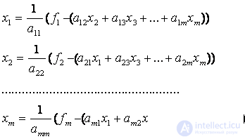(one),

Now, setting the zero approximation , according to the recurrence relations (1), we can perform an iterative process, namely:

(2)

Similarly, the following approximations are found. where in (2) instead of need to substitute .

Or in general:

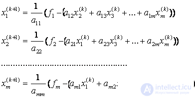. (3)

or

End condition of the iterative process .

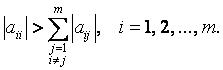
Sufficient condition of convergence: If the condition of diagonal dominance is satisfied, i.e. 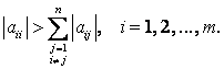, then the iterative process (3) converges with any choice of the initial approximation. If the original system of equations does not satisfy the condition of convergence, then it leads to a form with a diagonal predominance.

The choice of the initial approximation affects the number of iterations required to obtain an approximate solution. Most often, the initial approximation is taken 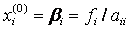or .

Remark The convergence condition indicated above is sufficient, i.e. if it is executed, the process converges. However, the process may converge in the absence of diagonal predominance, or it may not converge.

Example.

Solve a system of linear equations with precision :

	eight	four	2		ten		x 1
=	3	five	one	=	five	=	x 2
	3	–2	ten		four		x 3

Solution by direct methods, for example, an inverse matrix, gives a solution:

.

We will find a solution using simple iteration. Check the condition of diagonal dominance: , , .

We give the system of equations to the form (1):

.

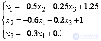Initial approximation . Further calculations will be arranged in the form of a table:

k	x 1	x 2	x 3	accuracy
0	0	0	0
one	1.250	1,000	0.400	1.2500
2	0.650	0.170	0.225	0.8300
3	1.109	0.565	0.239	0.4588
	………
four	0.908	0.287	0.180	0.2781
five	1.061	0.419	0.185	0.1537
6	0.994	0.326	0.165	0.0931
7	1.046	0.370	0.167	0.0515
eight	1.023	0.594	0.160	0.2235
9	0.913	0.582	0.212	0.1101
ten	0.906	0.505	0.242	0.0764
eleven	0.937	0.495	0.229	0.0305
12	0.945	0.516	0.218	0.0210
	……
13	0.937	0.523	0.220	0.0077

Here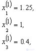

,

And so on, until we get, in the last column the value is less than 0.01, which will occur at the 13th iteration.

Therefore, the approximate solution is:

Gauss-Seidel Method

Calculation formulas are:

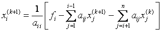
those. to calculate the i – th component of the ( k +1) –th approximation to the desired vector, the one already calculated on this is used, i.e. ( k +1) –th step, new values ​​of the first i –1 components .

Detailed formulas are:

A sufficient condition for the convergence of this method is the same as for the simple iteration method, i.e. diagonal dominance:

Initial approximation:

Let us find the solution of the previous system of equations by the Gauss – Seidel method.

Calculation formulas:

k	x1	x2	x3	accuracy
0	0	0	0
one	1.250	0.250	0.075	1.2500
2	1.106	0.321	0.132	0.1438
3	1.056	0.340	0.151	0.0500
four	1.042	0.344	0.156	0.0139
five	1.039	0.346	0.157	0.0036

The table shows that the required accuracy was reached already at the 5th iteration instead of the 13th using the simple iteration method and the root values ​​are closer to the values ​​obtained by the inverse matrix method.