3. Approximation of functions

Lecture

Local interpolation:
Piece-constant interpolation
Piecewise Linear Interpolation
Cubic interpolation spline
Global interpolation:
Polynom lagrange
Selection of empirical formulas
Least square method

Approximate - it means "to replace approximately." Suppose we know the values of some function at given points. It is required to find the intermediate values of this function. This is the so-called function recovery problem. In addition, when performing calculations, it is convenient to replace complex functions with algebraic polynomials or other elementary functions that are rather simply calculated ( the function approximation problem ).

Statement of the interpolation problem

On the interval [a, b] the points x _i , i = 0, 1, ..., N; a ≤ x _i ≤ b, and the values of the unknown function at these points are f _i , i = 0, 1, ...., N. It is required to find the function F (x) that takes the same values of f _i at points x _i . Points are called interpolation nodes , and the conditions F (x _i ) = f _i . - interpolation conditions . Moreover, we look for F (x) only on the segment [a, b]. If it is necessary to find a function outside the segment, then this is an extrapolation problem. For now, we will only consider interpolation tasks.

The task has many solutions, since through given points ( x _i , f _i ), i = 0, 1, ..., N, one can draw infinitely many curves, each of which will be a graph of a function for which all the interpolation conditions are satisfied. For practice, the important case is the approximation of a function by polynomials, i.e. .

All interpolation methods can be divided into local and global . In the case of local interpolation at each interval [ x _i– ₁ , x _i ] built a separate polynomial. In the case of global interpolation, a single polynomial is found over the entire interval [ a, b ] . In this case, the desired polynomial is called an interpolation polynomial .

Local interpolation

Piece-constant interpolation

On each segment the interpolation polynomial is equal to a constant, namely, the left or right value of the function.

For left piecewise linear interpolation i.e.

For the right piecewise linear interpolation i.e.

It is easy to understand that the interpolation conditions are satisfied. The constructed function is discontinuous), which limits its application. For the left piecewise linear interpolation, we have a graphical representation:

3. Approximation of functions

Piecewise Linear Interpolation

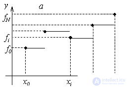
At each interval [ x _{i – 1} , x _i ] function is linear . The values of the coefficients are found from the fulfillment of the interpolation conditions at the ends of the segment: . We obtain the system of equations: , where do we find . Therefore, the function F (z) can be written in the form:

i.e.

Or F(x) = k _i * (x - x _i-1 ) + f _i-1 , k _i = (f _i - f _i-1 ) / (x _i - x _i-1 ), x _i-1 ≤ x ≤ x _i , i=1,2,...,N-1 F(x) = k _i * (x - x _i-1 ) + f _i-1 , k _i = (f _i - f _i-1 ) / (x _i - x _i-1 ), x _i-1 ≤ x ≤ x _i , i=1,2,...,N-1

When using linear interpolation, you must first determine the interval in which the value of x falls, and then substitute it into the formula.

The resulting function will be continuous, but the derivative will be discontinuous at each interpolation node. The error of such interpolation will be less than in the case of piecewise – constant interpolation. An illustration of the piecewise linear interpolation is shown in the figure.

3. Approximation of functions

Example: Some function values are given:

x	0	2	3	3.5
f	-one	0.2	0.5	0.8

It is required to find the value of the function at z = 1 and z = 3.2 by piecewise – constant and piecewise – linear interpolation.

Decision. Point z = 1 belongs to the first local segment [0, 2], i.e. and, therefore, according to the formulas of the left piecewise – constant interpolation F (1) = f ₀ = - 1 , according to the formulas of the right piecewise – interpolation constant F (1) = f ₁ = 0.2 . We use the piecewise linear interpolation formulas:

The point z = 3.2 belongs to the third interval [3, 3.5], i.e. and, therefore, according to the formulas of the left piecewise - constant interpolation F (3.2) = = 0.5, according to the formulas of the right piecewise - constant interpolation F (3.2) = = 0.8. We use the piecewise linear interpolation formulas:

Cubic interpolation spline

The word spline (the English word "spline") means a flexible ruler used to draw smooth curves through given points on a plane. The shape of this universal piece on each segment is described by a cubic parabola. Splines are widely used in engineering applications, in particular, in computer graphics. So, on each i –th segment [ x _i _–1 , x _i ] , i = 1, 2, ..., N, the solution will be sought in the form of a third degree polynomial:

S _i ( x ) = a _i + b _i ( x – x _i ) + c _i ( x - x _i ) 2/2 + d _i ( x – x _i ) 3/6

Unknown coefficients a _i , b _i , c _i , d _i , i = 1, 2, ..., N, we find from:

• interpolation conditions: S _i ( x _i ) = f _i , i = 1, 2, ..., N ; S ₁ ( x ₀ ) = f ₀ ,

• continuity of the function S _i ( x _i– ₁ ) = S _i– ₁ ( x _i _–1 ) , i = 2, 3, ..., N,

• continuity of the first and second derivative:

S ^/ _i ( x _i– ₁ ) = S ^/ _i– ₁ ( x _i _–1 ) , S ^// _i ( x _i _–1 ) = S ^// _i _–1 ( x _i _–1 ) , i = 2, 3, ..., N.

Considering that , to determine 4 N unknowns, we obtain a system of 4 N –2 equations:

a _i = f _i , i = 1, 2, ..., N,

b _i h _i - c _i h _i ^2/2 + d _i h _i 3/6 = f _i - f _i _–1 , i = 1, 2, ..., N,

b _i - b _{i – 1} = c _i h _i - d _i h _i 2/2 , i = 2, 3, ..., N,

d _i h _i = c _i - c _i– ₁ , i = 2, 3, ..., N.

where h _i = x _i - x _i– _{1 .} The missing two equations are derived from additional conditions: S ^// ( a ) = S ^// ( b ) = 0. It can be shown that in this case . The unknowns b _i , d _i can be excluded from the system by obtaining a system of N + 1 linear equations (SLAE) for determining the coefficients c _i :

c ₀ = 0 , c _N = 0,

h _i c _i _–1 + 2 ( h _i + h _i ₊₁ ) c _i + h _i ₊₁ c _i ₊₁ = 6 , i = 1, 2, ..., N –1 . (one)

After that, the coefficients b _i , d _i are calculated :

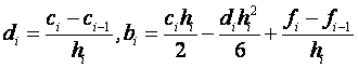, i = 1, 2, ..., N. (2)

In the case of grid constant h _i = h this the system of equations is simplified.

This SLAU has a three-diagonal matrix and is solved by the sweep method.

Coefficients are determined from the formulas:

To calculate the value of S ( x ) at an arbitrary point of the segment z ∈ [ a, b ], it is necessary to solve the system of equations for the coefficients c _i , i = 1,2, ..., N –1 , then find all the coefficients b _i , d _i . Further, it is necessary to determine which interval [ x _i _{0 ,} x _i _0–1 ] falls on this point, and, knowing the number i ₀ , calculate the value of the spline and its derivatives at the point z

S ( z ) = a _i ₀ + b _i ₀ ( z – x _i ₀ ) + c _i ₀ ( z – x _i ₀ ) 2/2 + d _i ₀ ( z – x _i ₀ ) 3/6

S ^/ ( z ) = b _i ₀ + c _i ₀ ( z – x _i ₀ ) + d _i ₀ ( z – x _i ₀ ) 2/2 , S ^// ( z ) = c _i ₀ + d _i ₀ ( z – x _i ₀ ) .

Example.

	x ₀ f ₀	x ₁ f ₁	x ₂ f ₂	x ₃ f ₃	x ₄ f ₄
x	0	¼	1/2	3/4	one
f	one	2	one	0	one

It is required to calculate the values of the function at points 0.25 and 0.8, using spline interpolation.

In our case: h _i = 1/4, .

We write the system of equations to determine :

Solving this system of linear equations, we get: .

Consider the point 0.25, which belongs to the first segment, i.e. . Therefore, we get

Consider point 0.8, which belongs to the fourth segment, i.e. .

Consequently,

Global interpolation

In the case of global interpolation, a single polynomial is found over the entire interval [ a, b ], i.e. a polynomial is constructed, which is used to interpolate the function f (x) over the entire interval of variation of the argument x. We will look for the interpolating function in the form of a polynomial (polynomial) of m –th power P _m ( x ) = a ₀ + a ₁ x + a ₂ x ² + a ₃ x ³ +… + a _m x ^m . What should be the degree of the polynomial in order to satisfy all interpolation conditions? Suppose that two points are given: ( x ₀ , f ₀ ) and ( x ₁ , f ₁ ), i.e. N = 1. A single straight line can be drawn through these points, i.e. the interpolating function is the first degree polynomial P ₁ ( x ) = a ₀ + a ₁ x. Through three points (N = 2) one can draw a parabola P ₂ ( x ) = a ₀ + a ₁ x + a ₂ x ² , etc. Reasoning in this way, we can assume that the desired polynomial must have degree N.

In order to prove this, we write out the system of equations for the coefficients. The equations of the system are the interpolation conditions in for each x = x _i :

This system is linear with respect to the desired coefficients a ₀ , a ₁ , a ₂ , ..., a _N. It is known that SLAE has a solution if its determinant is non-zero. The determinant of this system

bears the name of the determinant of Vandermond . From the course of mathematical analysis it is known that it is non-zero if x _k x _m (i.e., all interpolation nodes are different). Thus, it is proved that the system has a solution.

We showed that to find the coefficients
a ₀ , a ₁ , a ₂ , ..., a _N need to solve SLAE, which is a difficult task. But there is another way to construct a polynomial of the Nth degree, which does not require solving such a system.

Polynom lagrange

The solution is sought in the form where l _i ( z ) - basic polynomials N of degree for which the condition is satisfied: . Make sure that if such polynomials are constructed, then L _N ( x) will satisfy the interpolation conditions:

How to build basic polynomials ? Define

, i = 0, 1, ..., N.

Easy to understand that

, etc.

The function l _i ( z ) is a polynomial of the Nth degree of z and for it the conditions of "basicity" are satisfied:

= 0, i ≠ k ;, i.e. k = 1, ..., i-1 or k = i + 1, ..., N.

Thus, we managed to solve the problem of constructing an N – th degree interpolating polynomial, and for this we need not solve the SLAE. Polynomial Lagrange can be written in the form of a compact formula: . The error of this formula can be estimated if the original function g ( x ) has derivatives up to the N + 1 order:

From this formula it follows that the accuracy of the method depends on the properties of the function g ( x ) , as well as on the location of the interpolation nodes and the point z. As the calculated experiments show, the Lagrange polynomial has a small error for small values of N <20 . For larger N, the error begins to increase, which indicates that the Lagrange method does not converge (that is, its error does not decrease with increasing N ).

Consider special cases. Let N = 1, i.e. values of the function are given only at two points. Then the base polynomials are:

i.e. we obtain formulas of piecewise linear interpolation.

Let N = 2. Then:

As a result, we obtained the formulas of the so-called quadratic or parabolic interpolation.

Example: Some function values are given:

x	0	2	3	3.5
f	-one	0.2	0.5	0.8

It is required to find the value of the function at z = 1, using the Lgrange interpolation polynomial. For this case, N = 3, i.e. Lagrange polynomial has a third order. Calculate the values of the basis polynomials at z = 1 :

Selection of empirical formulas

When interpolating functions, we used the condition of equality of the values of the interpolation polynomial and this function at the interpolation nodes. If the initial data are obtained as a result of experimental measurements, then the exact match requirement is not necessary, since the data are not obtained accurately. In these cases, you can only require approximate fulfillment of the interpolation . This condition means that the interpolating function F ( x) passes not exactly through the given points, but in some of their neighborhoods, for example, as shown in Fig.

3. Approximation of functions

Then they talk about the selection of empirical formulas . The construction of an empirical formula consists of two stages6 the selection of the form of this formula containing unknown parameters , and the definition of the best in some sense of these parameters. The form of the formula is sometimes known from physical considerations (for elastic media, the relationship between stress and strain) or selected from geometrical considerations: the experimental points are plotted and the general form of the dependence is approximately guessed by comparing the curve obtained with the well-known functions. Success here is largely determined by the experience and intuition of the researcher.

For practice, the important case is the approximation of a function by polynomials, i.e. .

After the type of empirical dependence is chosen, the degree of closeness to the empirical data is determined using the minimum of the sum of squared deviations of the calculated and experimental data.

Least square method

Let for the initial data x _i , f _i , i = 1 , ..., N (numbering is better to start with unity), the type of empirical dependence is chosen: with unknown coefficients . We write the sum of the squares of the deviations between the empirical calculated values and the given experimental data:

Options we will find from the condition of the minimum function . This is the least squares method (least squares).

It is known that at the minimum point all partial derivatives of by are zero:

(one)

Consider the use of OLS for a particular case that is widely used in practice. As an empirical function, consider the polynomial

Formula (1) to determine the sum of squared deviations will take the form:

(2)

Calculate the derivatives:

Equating these expressions to zero and collecting coefficients for unknown , we obtain the following system of linear equations:

This system of equations is called normal. Solving this system of linear equations, we obtain the coefficients .

In the case of a first-order polynomial, m = 1, i.e. , the system of normal equations takes the form:

When m = 2, we have:

As a rule, choose several empirical dependencies. According to the OLS, the coefficients of these dependencies are found and among them they find the best by the minimum amount of deviations.

Example. The coordinates of the points are given:

x	-five	-3.5	-2	1.5	3.25	five
f	0.5	1.2	1.4	1.6	1.7	1.5

those. N = 6. It is required to find empirical dependencies: linear quadratic hyperbolic according to the OLS method and choose among them the best by the smallest sum of squared deviations.