1.4 The simplest call flow and its properties

The simplest call flow is called a stationary ordinary flow without aftereffect. The simplest call flow is completely determined and given by the probability of the receipt of exactly K calls in the time [0, t). Denote this probability by Pk (t) with K = 0.1, 2.3, ..., and t> 0. Find the expression for Pk (t):

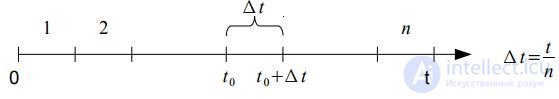
Consider the small time duration Δ t and calculate the probability that at least one call will be received during this time interval. By definition, the flow parameter we called the relationship limit:

Consequently, up to infinitesimally higher order, as Δ t → 0, it can be considered the probability that in the time Δ t there will be at least one call equal to:

and the probability that there will not be a single call equal to :

Since, by definition, the simplest flow is a flow without aftereffect, the probabilities of incoming calls in non-overlapping periods of time are independent. Therefore, n intervals of time can be considered as n independent experiments, in each of which the time interval Δ t can be “occupied” with probability λ⋅t / n.

The probability that among n intervals there will be exactly K "occupied" can be determined by the theorem on the repetition of experiments (according to the Bernoulli formula) from the expression

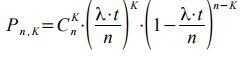
If n is sufficiently large, this probability is approximately equal to the probability of exactly K arriving at the time interval [0, t), since the probability of two or more calls arriving at the interval Δ t has a negligible probability (the simplest stream is ordinary!). To find the exact value

P k (t), you need to go to the limit as n → ∞:

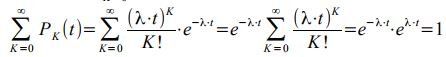
The probability distribution PK (t) is called the Poisson distribution. To verify that the sequence of probabilities PK (t) is a series of distributions, it is necessary to show that the sum of all probabilities PK (t) is equal to one. Indeed, based on the Maclaurin series

, we get:

To construct a Poisson distribution, it is necessary for all K to calculate PK (t). This is a distribution of a discrete random variable. When λ⋅t = 4, the distribution is as follows:

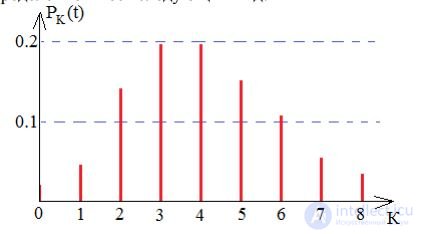
The envelope Poisson distributions for different λ⋅t have the following form:

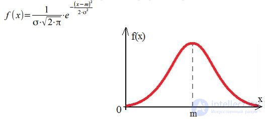
As can be seen from the figure, as the envelope grows, it becomes more and more symmetrical. When λ⋅t⩾10, there is a good agreement between the envelope of the Poisson distribution law and the normal distribution law (which is the distribution law of a continuous random variable), the formula and graph of which is: