Lecture
Determine the mathematical expectation of the number of calls arriving in time [0, t):
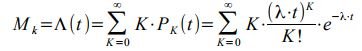
- expression of the initial moment of the first order.
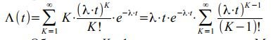
The first term of the sum at K = 0 is zero, therefore summation can be started with K = 1:
Denoting K − 1 = r, using the Maclaurin series, we obtain:
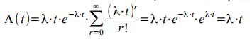
But on the other hand: Λ (t) = μ⋅t - by definition for a stationary flow. Therefore, for the simplest flow, the intensity is numerically equal to the parameter - μ = λ. The variance of a random variable distributed according to Poisson’s law will be determined from the expression:
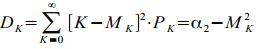
Where M k is the mathematical expectation, M k = Λ (t) = λ⋅t, α2 is the initial moment of the second order.
By definition:
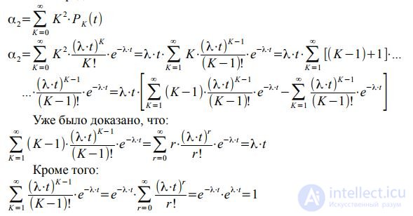
Consequently:
α2 = λ⋅t⋅ [λ⋅t + 1]
Dispersion of the simplest flow:
Dk = α2 − MK 2 = λ⋅t⋅ (λ⋅t + 1) - (λ⋅t) 2 = λ⋅t
Thus, the variance of the simplest call flow is equal to the expectation:
M k = Dk = λ⋅t
From this property of the simplest flow follows an important conclusion for practice: the relative variability of the simplest call flow is the smaller, the greater its mathematical expectation. Relative variability is estimated by the coefficient of variation, the ratio:
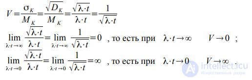
Consider two extreme cases: the limiting value at which the relative oscillation is zero (corresponds to the deterministic flow) and the second case as Δ t → 0 (the relative variability will increase indefinitely).
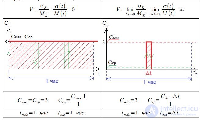
In the first case, with three lines of loss will not, and η = 100%,
where η = t Zan / t OBS.
In the second case, there will be no losses with three lines, but as Δ t → 0 η → 0.
η is the average use of channels
t obb - the duration of the observation,
t Zan - the duration of employment of one channel.
The higher the relative variability of the call flow, the lower the average utilization of channels in the beam with a fixed quality of service (P = const). This property of the flow explains the dependence:
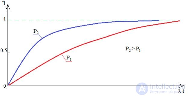
λ⋅t is the mathematical expectation of the number of calls coming in [0, t).
Hence, the efficiency of the telephone communication system is the higher, the greater the intensity of the incoming call flow to the system. This fundamental property of random call flows is widely used in queuing systems: in telecommunications, high-capacity telephone exchanges and switching nodes are built to concentrate the call flows; in trade - super-and hypermarkets; in transport - major airports and stations
Union and separation of independent simplest threads:
The union of independent simplest flows with parameters λ1, λ2, λ3, ..., λi, ..., λn will also be the simplest flow with parameter λ = ∑ λi equal to the sum of the parameters of the combined flows.
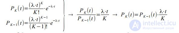
Poisson's recurrent formula:
Denote by t in - the average length of stay in the system of one call (usually accepted t in = 1). Divide and multiply t by t in:
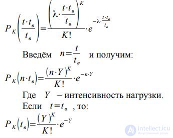
Given this, in order to more efficiently service call flows, it is desirable to merge them.
Without proof, we note another interesting property of the simplest flow: when summing a large number of independent ordinary stationary flows with almost any after-effect, we obtain a flow that is arbitrarily close to the simplest .
Analogy: “when summing up a large number of independent random variables, subordinate to virtually any distribution laws, we get a value that is approximately distributed according to the normal law”.

Comments
To leave a comment
Teletraffic Theory
Terms: Teletraffic Theory