Lecture
The Mills model is a method for estimating the number of errors in a program code, created in 1972 by programmer Harlan Mills. It is widespread due to its simplicity and intuitive appeal.
Suppose there is a program code in which there is a previously unknown number of errors (bugs)  requiring the most accurate assessment. To obtain this value, you can add to the program code
  additional errors, the presence of which is not known to specialists in testing [3] [1].
Suppose that after testing, n natural errors were detected (where n [1] [4]).
From which it follows that the estimate of the total number of natural errors in the code is equal to  , and the number of still not caught code bugs is equal to the difference
  [1] [5]. Mills himself believed that the testing process should be accompanied by constant updating of graphs to estimate the number of errors [6].
Obviously, this approach is not without flaws. For example, if 100% of artificial errors are found, then it means about 100% of natural errors were found. Moreover, the less artificial errors were made, the greater the likelihood that all of them will be detected. What follows is a deliberately absurd consequence: if only one error was introduced that was discovered during testing, it means there are no more errors in the code [6].
In order to quantify the confidence of the model, the following empirical criterion was introduced:

Significance level  estimates the probability with which the model will correctly reject the false assumption [7] [6]. Expression for It was constructed by Mills [7], but due to its empirical nature, if necessary, it allows for some variation within reasonable limits [8].
Based on the formula for You can get an estimate of the number of artificially introduced bugs. to achieve the desired confidence . This quantity is given by the expression  [eight].
The weakness of the Mills approach is the need to test the product before detecting absolutely all artificially introduced bugs, but there are generalizations of this model where this restriction is removed [7]. For example, if the threshold on the allowable number of detected errors is equal to  ), the criterion is overwritten as follows:

The statistical model of Mills allows us to estimate not only the number of errors before testing, but also the degree of smoothness of programs. To use the model prior to testing, errors are intentionally introduced into the program. Further, it is considered that the detection of intentionally introduced and so-called own program errors is equally probable.
To estimate the number of errors in the program before the start of testing, the expression is used
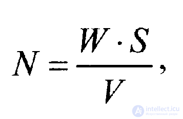 (2.2.1)
where W 'is the number of errors intentionally introduced into the program prior to testing; V is the number of errors from the number of intentionally introduced in the testing process; S is the number of "own" program errors detected during the testing process.
If we continue testing until all the errors intentionally detected are detected, the degree of smoothness of program C can be estimated using the expression
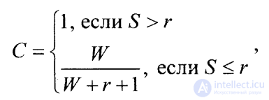 (2.2.2)
where S and W = V (equality of W and V values in this case takes place, since it is considered that all intentionally introduced errors are detected) have the same meaning as in the previous expression (2.2.1), and r means the upper limit (maximum) of the estimated number of "own" errors in the program.
Expressions (2.2.1) and (2.2.2) are the statistical model of Mills. It should be noted that if the testing is completed prematurely (that is, before all intentionally introduced errors are detected), then the more complex combinatorial expression (2.2.3) should be used instead of expression (2.2.2). If only V errors are detected from W intentionally introduced, the expression
 !!! (2.2.3)
where in parentheses are the notation for the number of combinations of S elements by V - 1 elements in each combination and the number of combinations of S + r + 1 elements by r + V elements in each combination.
Task 1
The program intentionally made (sowed) 10 errors. As a result of testing, 12 errors were detected, of which 10 errors were intentionally introduced. All found errors are corrected. Before testing, it was assumed that the program contains no more than 4 errors. It is required to estimate the number of errors before testing and the degree of smoothness of the program.
The solution of the problem
To estimate the number of errors before testing, use the formula (2.2.1).
We know:
• number of errors entered into the program W = 10;
• the number of detected errors among the entered V = 10;
• the number of "own" errors in the program S = 12 - 10 = 2.
Substituting these values in the formula, we obtain an estimate of the number of errors:
N = ( W · S ) / V = (10 · 2) / 10 = 2.
Thus, from the test results it follows that prior to the start of testing, there were 2 errors in the program.
To assess the smoothness of the program, use equation (2.2.2). We know:
• the number of detected "own" errors in the program S = 2;
• the number of expected errors in the program r = 4;
• the number of intentionally introduced and detected errors W = 10.
Obviously, a smaller number of “own” errors was detected than the number of expected errors in the program ( S< r ). To assess the smoothness of the program using the equation
C = W / ( W + r + 1) = 10 / (10 + 4 + 1) = 0.67.
The degree of smoothness of the program is 0.67, which is 67%.
Task 2
The program was intentionally introduced (sown) 14 errors. Suppose that the program before testing was 14 errors. During the four test runs, the following number of errors were identified.
|
Run number |
one |
2 |
3 |
four |
|
V |
6 |
four |
2 |
2 |
|
S |
four |
2 |
one |
one |
You must estimate the number of errors before each test run. Evaluate the degree of smoothness of the program after the last run. Build a diagram of the dependence of the possible number of errors in this program on the number of the test run.
The solution of the problem
The number of errors before each run will be estimated in accordance with expression (2.2.1). Before each subsequent evaluation of the number of errors and the degree of smoothness of the program, it is necessary to adjust the values of the entered W and estimated r errors taking into account the identified and eliminated after each test run.The degree of smoothness of the program on all runs, except the last (2.2.2), is calculated using the combinatorial formula (2.2.3).
When determining the program indicators based on the results of the first run, it is necessary to take into account that W 1 = 14; S 1 = 4; V 1 = 6, then
N 1 = ( W 1 · S 1) / V 1 = (14 · 4) / 6 = 9.
Before the second run, we adjust the source data for parameter estimation: r 2 = 14 - 4 = 10; W 2 = 14 - 6 = 8; S 2 = 2; V 2 = 4, then
N 2 = ( W 2 · S 2) / V 2 = (8 · 2) / 4 = 4.
Adjusting the source data before the third run gives the following data. r 3 = 10 - 2 = 8, W 3 = 8 - 4 = 4; S 3 = 1; V 3 = 2, where the number of errors is determined as follows:
N 3 = ( W 3 · S 3) / V 3 = (4 · 1) / 2 = 2.
Before the fourth program run, we get the following initial data: r 4 = 8 - 1 = 7, W 4 = 4 - 2 = 2; S 4 = 1; V 4 = 2, then
N 4 = ( W 4 · S 4) / V 4 = (2 · 1) / 2 = 1.
Since after the fourth run all the “sown” errors were identified and eliminated, then to evaluate the smoothness of the program, you can use the simplified formula
C = W / ( W + r + 1) = 2 / (2+ 7+ 1) = 0.2.
Thus, under the assumption that before the fourth run, 7 errors remained in the program, the degree of program smoothness is 20%.
The result of the number of errors in the program before the start of each run is given below.
|
Run number |
one |
2 |
3 |
four |
|
N |
9 |
four |
2 |
one |

Comments
To leave a comment
Quality Assurance
Terms: Quality Assurance