Lecture
Operational calculus is one of the methods of mathematical analysis, which in a number of cases allows us to solve complex mathematical problems using very simple tools.
In the middle of the XIX century, a number of works appeared on the so-called symbolic calculus and its application to the solution of certain types of linear differential equations. The essence of symbolic calculus is that the functions of the differentiation operator are introduced and properly interpreted  (see Operator calculus). Among the essays on symbolic calculus should be noted published in 1862 in Kiev, a thorough monograph of the Ukrainian mathematician M. Ye. Vaschenko-Zakharchenko “Symbolic calculus and its application to the integration of linear differential equations”. It sets and resolves the main tasks of the method, which later became known as the operating method.
In 1892, the works of the English scientist O. Heaviside appeared, devoted to the application of the method of symbolic calculus to solving problems in the theory of the propagation of electrical oscillations in wires. Unlike his predecessors, Heaviside defined the inverse operator uniquely, assuming 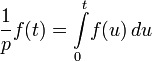 and counting
  for
for  . Heaviside's works laid the foundation for the systematic application of symbolic, or operational, calculus to the solution of physical and technical problems.
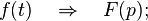
However, the operational calculus widely developed in the Heaviside writings did not receive a mathematical justification, and many of its results remained unproved. The rigorous justification was given much later, when the link between the functional Laplace transform was established 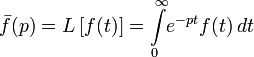 and differentiation operator
  Namely, if there is a derivative
  , for which
  exists and
  then
then 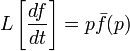
Operational calculus is a method of integrating some classes of linear differential equations, which consists in first looking for the unknown function itself, which satisfies the differential equation, and some corresponding option, transformed by Laplace. This method is also directly used to solve some types of linear partial differential equations, as well as difference, differential-difference equations, and some types of integral equations.
The construction of operational calculus is based on the idea of transforming a function of a real variable t, which is called the original, into a function of a complex variable p, which is called an image.
The original of the linear combination of functions is equal to the linear combination of images with the same coefficients.

where a and b are arbitrary complex numbers.
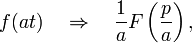
where a> 0.


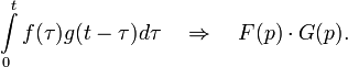
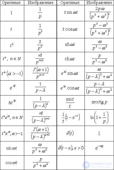
| Original | Picture | Original | Picture | Original | Picture | ||
|---|---|---|---|---|---|---|---|
 |
 |
 |
 |
 |
 |
||
 |
 |
 |
 |
 |
 |
||
 |
 |
 |
 |
 |
 |
||
 |
 |
 |
 |
 |
 |
||
 |
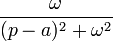 |
 |
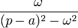 |
 |
 |
||
 |
 |
 |
 |
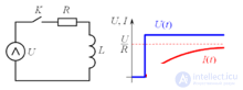
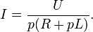
The figure shows a switched RL chain. At some time t = 0, the key K closes. Determine the dependence of the current in the RL-chain from time to time.
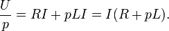
According to the second Kirchhoff law, the scheme is described by the following differential equation:
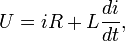
where the first term describes the voltage drop across the resistor R, and the second to the inductance L.
We do variable replacement  and reduce the equation to the form:

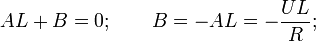
Since one of the factors a, b can be chosen arbitrarily, we choose b so that the expression in parentheses is zero:
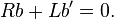
Separate variables:
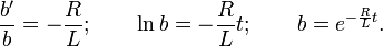
Given the chosen value of b, the differential equation is reduced to the form
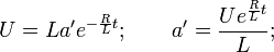
Integrating, we get
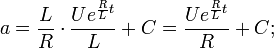
We get the expression for the current
The value of the integration constant is found from the condition that at the time t = 0 there was no current in the circuit:
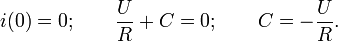
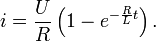
Finally we get
Find images of each of the components of the differential equation:
 [one]
[one]
 is obtained because the change in U in time is expressed by the function U = H (t) U (the key is closed at the time t = 0), where H (t) is a Heaviside step function, ( H (t) = 0 for t <0 and H (t) = 1 at t = 0 and t > 0, and the image H (t) is 1 / p ).
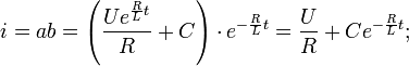
We get the following image of the differential equation
From the last expression we find the current image:
Thus, the solution is reduced to finding the original current in a known image. We decompose the right side of the equation into elementary fractions:


Find the originals of the elements of the last expression:
Finally we get
Operational calculus is extremely convenient in electrical engineering for calculating the dynamic modes of various circuits. The algorithm for calculating the following.
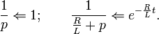
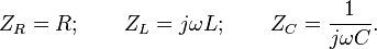
1) All elements of the circuit are considered as resistances Z i , the values of which are found on the basis of images of transition functions of the corresponding elements.
For example, for a resistor:

For inductance:
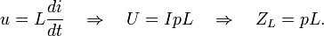
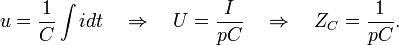
For capacity:
2) Using the specified resistance values, we find the images of the currents in the circuit, using standard methods of calculating circuits used in electrical engineering.
3) Having images of currents in the circuit, we find the originals, which are the solution of the differential equations describing the circuit.
It is interesting to note that the expressions obtained above for the operator resistance of various elements with accuracy up to

coincide with the corresponding expressions for resistances in AC circuits:

Comments
To leave a comment
Comprehensive analysis and operational calculus
Terms: Comprehensive analysis and operational calculus