Lecture
Herglotz theorem. Formulation of the Bochner-Khinchin Theorem

§ 9. As the title of the chapter suggests, our main interest is related to consideration.
stationary processes. It turns out that the above Karunen theorem,
applied to such processes, allows us to obtain stochastic assumptions for them.
statements that allow for a very transparent "spectral" interpretation.
Recall that the essence of the concept of stationarity of a random process is that
that the statistical characteristics of such a process are invariant with respect to
shifts t n-> ¦ t + and. This needs clarification. First of all, to have
the ability to shift the argument t of the process being studied X = {X (t),
t G T}, it is assumed that T is a certain group (everywhere, by addition).
As a temporary set of T, as a rule, many
b) - {0, = Ы, ...} or Е = (_Loo, оо), which corresponds to the study of processes
with discrete or continuous time. In addition, the values of X (t) for each
t G T are considered to belong to the same space S (usually S = С
orB = E).
Definition 8 of Chapter VI of a stationary in the narrow sense of the process is preserved
for the case when T is a group.
Many studies are interesting properties of random processes,
depending only on the mixed moments of certain orders, that is, on the functions
of the form EX (ti) kl • • • X (tn) kn, where n GN, ti, ..., tn G G, fci, ..., kn G Z +. For class
L2 processes this makes it natural.
Definition 6. Complex-valued (in particular, real) L2-npo-
the process X = {X (t), t ∈ T}, where T is a certain group, is called stationary
broadly (or stationary second order) if
EX (t) = a for any t ∈ Γ, B4)
r (s, t) = cov (X (s), X (t)) = r (s ± t, 0) (: = R (s ± t)) for all s, teT. B5)
It is easy to see that any stationary in the narrow sense L2-nponecc will be a
stationary in a broad sense. For Gaussian processes, these concepts coincide.
A sequence of independent identically distributed quantities that do not have
expectation, gives an example of a stationary in the narrow sense of the process,
for which it is meaningless to talk about stationarity in a broad sense.
Next we focus on processes that are stationary in a broad sense. Theory
of such processes is closely connected with the theory of curves in the Hilbert space and
with the property of non-negative definiteness of deterministic functions.
Definition 7. The complex-valued function R = R (t), t ∈ T, given on a non-
which group T is called non-negative definite, if non-negative
but the function r (s, t) = R (s _L t) is defined, s, t GT, i.e., condition A1.13) holds.
It follows from Theorem 4 of Chapter II that the class of non-negative definite functions
R = R (t), t ∈ T, where T is a group, coincides with the class of covariance functions
stationary Gaussian processes X = {X (?),? G T}.
Description of non-negative definite functions on the group T = b - {0, = Ы, ...}
gives the following
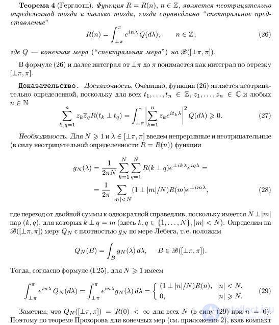
Theorem 4 (Herglotz). The function R = R (n), n GZ, is non-negative
determined if and only if the "spectral representation
setting "
R (n) = f einXQ (d \), ne6, B6)
J ± 7T
where Q is a finite measure ("spectral measure") on J§ ([_ 1_tg, tg]).
In the formula B6) and further the integral from _1_tg to tg is understood as the integral over the segment
[J-tt.tt].
Proof. Adequacy. Obviously, the function B6) is non-negative
defined, since for all t \, ..., tn GZ, z \, ..., zn G C any
ne N
2
J] * kZq.
k, q = l
Q (d \) ^ 0. B7)
Need. For TV ^ 1 and AG [_Ltt, tg], we introduce continuous and non-negative
(due to non-negative definiteness R = R (n)) functions
B8)
\ m \ <N
where the transition from double to one-time is fair, since there is iV _L | yyy |
pairs (k, q) for which k _L q = m (here k, q G {1, ..., N}, \ m \ <N). Define on
_7r, tg]) measure Qn with density gjsf as Lebesgue measure, i.e., we set
QN (B) = / gN (X) d \, B e 58 ([J_7r, 7r]).
Jb
b
Then, according to formula A.25), for N ^ 1 we have
i_L7r i_L7r
Note that Qiv ([_ L7r, 7r]) = R @) <oo for all N (by virtue of B9) with n = 0).
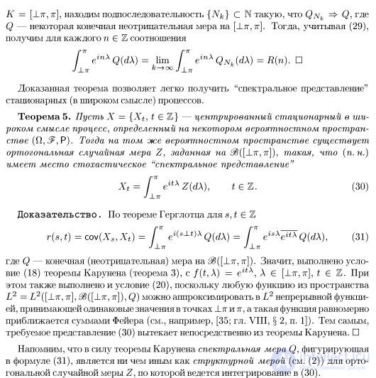
Therefore, by Prokhorov’s theorem for finite measures (see Appendix 2), taking the compact
K = [_Ltt, tt], we find a subsequence {N ^} С N such that Qnu => Q-, where
Q is some finite non-negative measure on [_1_tg, ng]. Then, considering B9),
get for each p E Z ratio
Г einXQ (d \) = lim G einXQNk (d \) = R (n). D
Proved theorem makes it easy to get a "spectral representation"
stationary (in a broad sense) processes.
Theorem 5. Let X = {Xf, t GZ} be centered stationary in
In the extreme sense, a process defined on a certain probability space
(P, ^, P). Then on the same probability space there is
the orthogonal random measure Z given on §§ ([_ 1_tg, tg]), such that (n.)
there is a stochastic "spectral representation"
Xt = [eitxZ (dX), te%. C0)
Evidence. According to the Herglotz theorem for s, tGZ
s, t) = cov (XSjXt) = Г e ^ s ± t ^ xQ (dX) = Г eisX ^ Q (dX), C1)
J ± 7T J ± 7T
where Q is a finite (nonnegative) measure on ^ ([_ Ltt, ng]). So, the condition
Vii A8) of the Karunen theorem (Theorem 3), with / (t, A) = eltx, XG [_Ltt, ng], t G Z. With
this also fulfills the condition B0), since any function from the space
L2 = L2 ([_ Ltt, ng], ^ ([_ Ltt, ng]), Q) can be approximated in L2 continuous function
to it, taking the same values at the points _Ltt and n, and such a function is uniform
approximates by the Fejér sums (see, for example, [35; chap. VIII, § 2, paragraph 1]). Thereby,
the required representation C0) follows directly from the Karhunen theorem. ?
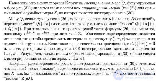
Recall that by virtue of the Karunen theorem, the spectral measure Q that appears
in formula C1) is nothing more than a structural measure (see B)) for the ortho-
zonal random measure Z, which is integrated into C0).
The measure Q used in B6) can be redefined (without changing the notation),
transferring the "mass" Q ({_ Ltt}) from the point _Ltt to the point m, where the "mass" Q ({_ Ltt}) will appear +
+ Q ({tt}). The value of the integral in the right side of the formula B6) does not change,
since e ± hP7T = erP7T for all n G Z. The indicated redefinition is made
only in order to represent the integral over the interval (_1_tg, тг] as the integral over
unit circle. If such a mass transfer is made, then Z ({_ Ltt}) = 0
b.p. by virtue of Theorem 2, therefore, in C0) the integration is actually carried out by
(J_tt, ng]. Of course, the integration in C0 in a similar way) can be reduced
to the integration over the interval [_1_tg, m).
Concluding consideration of the issue of the spectral representation of C0), we note
that this (“spectral”) terminology is inspired by the fact that (according to C0))
Xt’s perceptions, as it were, are added up from the elXt spectral harmonics with
weights Z (dX).
§ 12. Description of covariance functions of stationary (in a broad sense) pro-
Cesses that are continuous in the mean square on T = E are given by the following
Theorem 8 (Bochner-Hinchin). Let R = R (t), t GE, be continuous at zero
non-negative definite function. Then for any t ∈ E
goo
R (t) = / eitxG (d \), C6)
where G = G (d \) is some non-negative finite ("spectral") metric
ra 3 & (W).
Obviously, the function defined by the right part of C6) is continuous on
all straight. Completely analogous to B7) make sure that she is also non-denying
well defined. Thus, the conditions of Theorem 8 are necessary. Evidence
sufficiency of these conditions is listed in Appendix 4.

Comments
To leave a comment
probabilistic processes
Terms: probabilistic processes