Teaching with the teacher (English Supervised learning ) is one of the methods of machine learning, during which the test system is forcibly trained using examples of "stimulus-response". From the point of view of cybernetics, is one of the types of cybernetic experiment. There may be some dependence between inputs and reference outputs (stimulus-response), but it is not known. Only a finite set of precedents is known — the stimulus-response pairs, called the training set . Based on these data, it is required to restore the dependence (build a model of stimulus-response relationships suitable for prediction), that is, to build an algorithm capable of producing a reasonably accurate answer for any object. To measure the accuracy of the answers, as well as in the example training, the quality functional can be introduced.

Content

• 1 The principle of this experiment
• 2 Typology of learning tasks with a teacher
  • 2.1 Types of input data
  • 2.2 Types of responses
• 3 Degenerate types of reinforcement management systems (“teachers”)
• 4 See also
• 5 Literature

The principle of this experiment

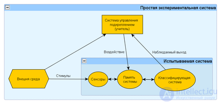
This experiment is a special case of a cybernetic experiment with feedback. The formulation of this experiment implies the existence of an experimental system, a training method, and a method for testing a system or measuring characteristics.

The experimental system, in turn, consists of the test (used) system, the space of stimuli obtained from the external environment and the reinforcement control system (regulator of internal parameters). As a reinforcement management system, an automatic regulating device (for example, a thermostat) or a human operator ( teacher ) can be used to respond to the reactions of the system under test and the external stimuli by applying special reinforcement rules that change the state of the system’s memory.

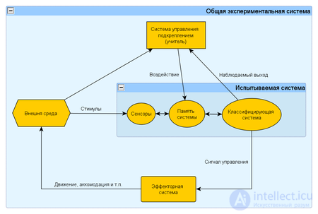
There are two options: (1) when the reaction of the system under test does not change the state of the external environment, and (2) when the system’s reaction changes the stimuli of the external environment. These schemes indicate the fundamental similarity of such a system of a general form with the biological nervous system.

Typology of learning tasks with a teacher

Types of input data

• The feature description is the most common case. Each object is described by a set of its characteristics, called attributes . Attributes can be numeric or non-numeric.
• Matrix of distances between objects. Each object is described by distances to all other objects of the training set. Few methods work with this type of input data, in particular, the method of the nearest neighbors, the parzen window method, the method of potential functions.
• The time series or signal is a sequence of measurements in time. Each dimension can be represented by a number, a vector, and in the general case - a characteristic description of the object under study at a given time.
• Image or video series.
• There are also more complex cases where the input data is presented in the form of graphs, texts, database query results, etc. As a rule, they are reduced to the first or second case by preprocessing the data and extracting the signs.

Types of responses

• When the set of possible answers is infinite (the answers are real numbers or vectors), they talk about regression and approximation problems;
• When a lot of possible answers of course, they talk about the tasks of classification and pattern recognition;
• When answers characterize the future behavior of a process or phenomenon, they talk about forecasting tasks.

Degenerate types of reinforcement management systems (“teachers”)

• The reinforcement system with reaction control ( R is a controlled system ) is characterized by the fact that the information channel from the external environment to the reinforcement system does not function. This system, despite the presence of a control system, refers to spontaneous learning, since the system under study is trained autonomously, under the action of only its output signals, regardless of their “correctness”. With this training method, no external information is required to control the change in the state of the memory;
• The reinforcement system with incentive management ( S - controlled system ) - is characterized by the fact that the information channel from the system under test to the reinforcement system does not function. Despite the non-functioning channel from the outputs of the system under test, it refers to training with a teacher, as in this case the reinforcement system (teacher) forces the system under test to develop reactions according to a certain rule, although the true reactions of the system under test are not taken into account.

This distinction allows for a deeper look at the differences between different ways of learning, since the line between teaching with a teacher and learning without a teacher is more subtle. In addition, this distinction made it possible to show for artificial neural networks certain restrictions for S and R-controlled systems (see Perceptron Convergence Theorem).

Error correction method

This article is about neural networks; For information error correction in computer science, see: Error detection and correction.

Error correction method is the perceptron learning method proposed by Frank Rosenblatt. It is a learning method in which the weight of a bond does not change as long as the current reaction of the perceptron remains correct. If an incorrect reaction appears, the weight changes by one, and the sign (+/-) is determined opposite to the error sign.

Content

• 1 Method Modifications
  • 1.1 Method of error correction without quantization
  • 1.2 Method of error correction with quantization
  • 1.3 Error correction method with random reinforcement sign
  • 1.4 Method of error correction with random disturbances
• 2 See also
• 3 Literature

Method modifications

In the perceptron convergence theorem, different types of this method differ, it is proved that any of them allows to obtain convergence when solving any classification problem.

Error correction method without quantization

If the response to the stimulus correct, no reinforcement is entered, but if errors occur, the value of each active A-element is added where - the number of reinforcement units, is chosen so that the magnitude of the signal exceeds the threshold θ, and 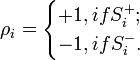, wherein - an incentive belonging to the positive class, and - an incentive belonging to the negative class.

Quantization Error Correction Method

It differs from the error correction method without quantization only in that , i.e. equal to one reinforcement unit.

This method and the method of error correction without quantization are the same in terms of the speed at which the solution is reached in the general case, and more effective than the error correction methods with a random sign or random perturbations .

Random error correction method

Differs in that reinforcement sign It is chosen randomly, regardless of the reaction of the perceptron, and with equal probability can be positive or negative. But just like in the base method - if the perceptron gives the right response, then the reinforcement is zero.

Method of error correction with random disturbances

Differs in that the magnitude and sign for each connection in the system are selected separately and independently in accordance with a certain probability distribution. This method leads to the slowest convergence compared to the modifications described above.

Error back propagation method

.

The method of back propagation of error (eng. Backpropagation ) is a method of teaching a multilayer perceptron. The method was first described in 1974. А.I. Galushkin [1] , as well as independently and simultaneously by Paul J. Verbos [2] . Further, it was substantially developed in 1986 by David I. Rumelhart, J. E. Hinton and Ronald J. Williams [3] and independently and simultaneously by S.I. Bartsevym and V.A. Okhonin (Krasnoyarsk group) [4] .. This is an iterative gradient algorithm that is used to minimize the error of the multilayer perceptron and to obtain the desired output.

The main idea of ​​this method is to propagate error signals from the network outputs to its inputs, in the opposite direction to direct signal propagation in normal operation. Bartsev and Okhonin immediately proposed a general method (“duality principle”) applicable to a wider class of systems, including delay systems, distributed systems, etc. [5]

To be able to apply the method of back propagation of error, the transfer function of neurons must be differentiable. The method is a modification of the classical gradient descent method.

Content

• 1 Sigmoidal activation function
• 2 Network evaluation function
• 3 Description of the algorithm
• 4 Algorithm
• 5 Mathematical interpretation of learning neural network
• 6 Disadvantages of the algorithm
  • 6.1 Network paralysis
  • 6.2 Local minima
  • 6.3 Step Size
• 7 See also
• 8 Literature
• 9 References
• 10 Notes

Sigmoidal activation functions

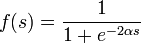
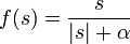
Most often, the following sigmoid types are used as activation functions:

Fermi function (exponential sigmoid):

Rational sigmoid:

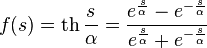
Hyperbolic Tangent:

,

where s is the output of the neuron adder, Is an arbitrary constant.

Least of all, compared with other sigmoids, processor time requires the calculation of a rational sigmoid. The calculation of the hyperbolic tangent requires the most cycles of the processor. If compared with threshold activation functions, then sigmoids are calculated very slowly. If, after summation in the threshold function, you can immediately begin a comparison with a certain value (threshold), then in the case of a sigmoidal activation function, you need to calculate sigmoid (spend time at best on three operations: taking the module, addition and division), and only then compare it with the threshold value (for example, zero). If we assume that all the simplest operations are calculated by the processor for approximately the same time, then the operation of the sigmoidal activation function after the summation performed (which takes the same time) will be slower than the threshold activation function as 1: 4.

Network evaluation function

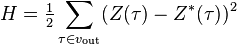
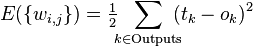
In cases where it is possible to evaluate the operation of the network, the training of neural networks can be represented as an optimization problem. To evaluate means to quantify whether the network solves its tasks well or badly. For this purpose, an evaluation function is built. As a rule, it obviously depends on the output signals of the network and implicitly (through functioning) on ​​all its parameters. The simplest and most common example of evaluation is the sum of the squares of the distances from the output signals of the network to their required values:

,

Where - the desired value of the output signal.

The method of least squares is not always the best choice of assessment. Careful design of the evaluation function allows an order of magnitude increase in the effectiveness of network training, as well as obtaining additional information - the “level of confidence” of the network in the response given [6] .

Algorithm Description

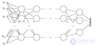
Multi-layer perceptron architecture

The backpropagation algorithm is applied to a multilayer perceptron. The network has multiple inputs. , multiple Outputs outlets and many internal nodes. Renumber all nodes (including inputs and outputs) with numbers from 1 to N (through numbering, regardless of the topology of the layers). Denote by the weight standing on the edge connecting the i th and j th nodes, and through - output of the i-th node. If we know the training example (the correct answers are , ), the error function obtained by the least squares method looks like this:

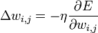
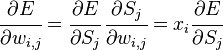
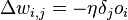
How to modify the weight? We will implement a stochastic gradient descent, that is, we will correct the weights after each training example and, thus, “move” in the multidimensional space of weights. To "get" to the minimum of error, we need to "move" in the direction opposite to the gradient, that is, based on each group of correct answers, add to each weight

,

Where - a factor that sets the speed of "movement".

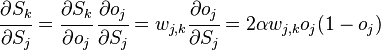
The derivative is calculated as follows. Let first , that is, the weight of interest to us is included in the neuron of the last level. First, we note that affects network output only as part of the amount 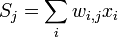where the sum is taken at the inputs of the jth node. therefore

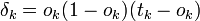
Similarly affects the total error only within the jth node output (recall that this is the output of the entire network). therefore

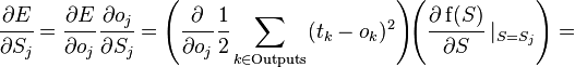
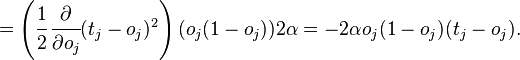
Where - the corresponding sigmoid, in this case - exponential

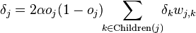
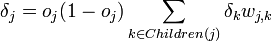
If the j- th node is not at the last level, then it has exits; we denote them by Children ( j ). In this case

,

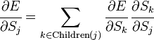and

.

well and - this is exactly the same correction, but calculated for the next level node we will denote it by - from it is distinguished by the absence of a multiplier . Поскольку мы научились вычислять поправку для узлов последнего уровня и выражать поправку для узла более низкого уровня через поправки более высокого, можно уже писать алгоритм. Именно из-за этой особенности вычисления поправок алгоритм называется алгоритмом обратного распространения ошибки (backpropagation). Краткое резюме проделанной работы:

• для узла последнего уровня

• для внутреннего узла сети

• для всех узлов

where это тот же в формуле для

Получающийся алгоритм представлен ниже. На вход алгоритму, кроме указанных параметров, нужно также подавать в каком-нибудь формате структуру сети. На практике очень хорошие результаты показывают сети достаточно простой структуры, состоящие из двух уровней нейронов — скрытого уровня (hidden units) и нейронов-выходов (output units); каждый вход сети соединен со всеми скрытыми нейронами, а результат работы каждого скрытого нейрона подается на вход каждому из нейронов-выходов. В таком случае достаточно подавать на вход количество нейронов скрытого уровня.

Algorithm

Алгоритм: BackPropagation

1. Инициализировать маленькими случайными значениями,
2. Повторить NUMBER_OF_STEPS раз:

   Для всех d от 1 до m:

   1. Подать на вход сети и подсчитать выходы каждого узла.
   2. For all

      .

   3. Для каждого уровня l, начиная с предпоследнего:

      Для каждого узла j уровня l вычислить

      .

   4. Для каждого ребра сети {i, j}

      .

      .

3. Выдать значения .

Where — коэффициент инерциальнности для сглаживания резких скачков при перемещении по поверхности целевой функции

Математическая интерпретация обучения нейронной сети

На каждой итерации алгоритма обратного распространения весовые коэффициенты нейронной сети модифицируются так, чтобы улучшить решение одного примера. Таким образом, в процессе обучения циклически решаются однокритериальные задачи оптимизации.

Обучение нейронной сети характеризуется четырьмя специфическими ограничениями, выделяющими обучение нейросетей из общих задач оптимизации: астрономическое число параметров, необходимость высокого параллелизма при обучении, многокритериальность решаемых задач, необходимость найти достаточно широкую область, в которой значения всех минимизируемых функций близки к минимальным. В остальном проблему обучения можно, как правило, сформулировать как задачу минимизации оценки. Осторожность предыдущей фразы («как правило») связана с тем, что на самом деле нам неизвестны и никогда не будут известны все возможные задачи для нейронных сетей, и, быть может, где-то в неизвестности есть задачи, которые несводимы к минимизации оценки. Минимизация оценки — сложная проблема: параметров астрономически много (для стандартных примеров, реализуемых на РС — от 100 до 1000000), адаптивный рельеф (график оценки как функции от подстраиваемых параметров) сложен, может содержать много локальных минимумов.

Недостатки алгоритма

Несмотря на многочисленные успешные применения обратного распространения, оно не является панацеей. Больше всего неприятностей приносит неопределённо долгий процесс обучения. В сложных задачах для обучения сети могут потребоваться дни или даже недели, она может и вообще не обучиться. Причиной может быть одна из описанных ниже.

Паралич сети

В процессе обучения сети значения весов могут в результате коррекции стать очень большими величинами. Это может привести к тому, что все или большинство нейронов будут функционировать при очень больших значениях OUT, в области, где производная сжимающей функции очень мала. Так как посылаемая обратно в процессе обучения ошибка пропорциональна этой производной, то процесс обучения может практически замереть. В теоретическом отношении эта проблема плохо изучена. Обычно этого избегают уменьшением размера шага η, но это увеличивает время обучения. Различные эвристики использовались для предохранения от паралича или для восстановления после него, но пока что они могут рассматриваться лишь как экспериментальные.

Локальные минимумы

Обратное распространение использует разновидность градиентного спуска, то есть осуществляет спуск вниз по поверхности ошибки, непрерывно подстраивая веса в направлении к минимуму. Поверхность ошибки сложной сети сильно изрезана и состоит из холмов, долин, складок и оврагов в пространстве высокой размерности. Сеть может попасть в локальный минимум (неглубокую долину), когда рядом имеется гораздо более глубокий минимум. В точке локального минимума все направления ведут вверх, и сеть неспособна из него выбраться. Основную трудность при обучении нейронных сетей составляют как раз методы выхода из локальных минимумов: каждый раз выходя из локального минимума снова ищется следующий локальный минимум тем же методом обратного распространения ошибки до тех пор, пока найти из него выход уже не удаётся.

Размер шага

Внимательный разбор доказательства сходимости [3] показывает, что коррекции весов предполагаются бесконечно малыми. Ясно, что это неосуществимо на практике, так как ведёт к бесконечному времени обучения. Размер шага должен браться конечным. Если размер шага фиксирован и очень мал, то сходимость слишком медленная, если же он фиксирован и слишком велик, то может возникнуть паралич или постоянная неустойчивость. Эффективно увеличивать шаг до тех пор, пока не прекратится улучшение оценки в данном направлении антиградиента и уменьшать, если такого улучшения не происходит. П. Д. Вассерман [7] описал адаптивный алгоритм выбора шага, автоматически корректирующий размер шага в процессе обучения. В книге А. Н. Горбаня [8] предложена разветвлённая технология оптимизации обучения.

It should also be noted the possibility of retraining the network, which is rather the result of an erroneous design of its topology. With too many neurons, the network property is lost to generalize information. The entire set of images provided for training will be learned by the network, but any other images, even very similar ones, may be classified incorrectly.