Lecture
Two basic computer architectures — sequential processing of characters from a given program and parallel pattern recognition from teaching examples — appeared almost simultaneously.
Conceptually, they took shape in the 30s-40s. The first is in the theoretical work of Turing in 1936, who proposed a hypothetical machine for formalizing the concept of a computable function, and then, in a practical way, generalized the lessons of creating the first ENIAC computer and proposed a methodology for designing machines with memorized programs (ENIAC was programmed with plugs). So, von Neumann proposed modified formal neurons by McCulloch and Pitts, the founders of neural network architecture, as basic elements of a computer.
As for the neural network architecture, despite the numerous overtures to the neural networks from the side of the cybernetics classics, their influence on industrial developments until recently was minimal. Although in the late 1950s and early 1960s, great hopes were pinned on this direction, mainly due to Frank Rosenblatt, who developed the first neural network pattern recognition device, the perceptron (from English perception, perception).
Perceptron was first modeled in 1958, and its training required about half an hour of computer time on one of the most powerful IBM-704 computers at that time. The hardware version - Mark I Perceptron - was built in 1960 and was designed to recognize visual images. His receptor field consisted of a 20x20 array of photodetectors, and he successfully coped with the solution of a number of problems.
At the same time, the first commercial neurocomputing companies appeared. In 1969, Marvin Minsky published a book entitled Perceptrons with the South African mathematician Papert. In this fatal book for neurocomputing, the fundamental limitations of perceptrons were strictly proved. Research in this direction was curtailed until 1983, when they finally received funding from the United States Agency for Advanced Military Research (DARPA). This fact was the signal for the start of a new neural network boom.
The interest of the general scientific community to neural networks has awakened after the theoretical work of the physicist John Hopfield (1982), who proposed a model of associative memory in neural ensembles. Holfield and his numerous followers have enriched the theory of neural networks with many ideas from the physics arsenal, such as collective interactions of neurons, network energy, learning temperature, etc. However, the real boom of practical use of neural networks began after the publication in 1986 by David Rumelhart and co-authors of the teaching method of a multi-layer perceptron, which they called the error back-propagation method. The perceptron limitations that Minsky and Papert wrote about turned out to be surmountable, and the capabilities of computing technology are sufficient to solve a wide range of applied problems. In the 90s, the productivity of serial computers increased so much that it allowed us to simulate the work of parallel neural networks with the number of neurons from several hundred to tens of thousands. Such neural network emulators are capable of solving many interesting problems from a practical point of view.
Artificial neural networks are based on the following features of living neural networks, allowing them to cope well with irregular tasks:
simple processing element - neuron (Fig.1.1);
a very large number of neurons involved in information processing;
one neuron is associated with a large number of other neurons (global connections);
weight-changing connections between neurons;
massive parallel processing of information.
The biological neuron of the brain served as a prototype for creating a neuron. A biological neuron has a body, a set of processes - dendrites, through which input signals enter the neuron, and a process - an axon, which transmits the output signal of the neuron to other cells. The junction point of the dendrite and the axon is called a synapse. Simplified functioning of the neuron can be represented as follows (Fig. 1.2):
1) the neuron receives from the dendrites a set (vector) of input signals;
2) in the body of the neuron is estimated the total value of the input signals.
However, the inputs of the neuron are unequal. Each input is characterized by a certain weighting factor, which determines the importance of the information received on it.
Thus, the neuron does not simply sum the values of the input signals, but calculates the scalar product of the vector of input signals and the vector of weight coefficients;

Fig.1.1 Biological neuron
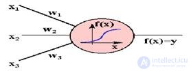
Fig.1.2 Artificial neuron
3) the neuron generates an output signal, the intensity of which depends on the value of the calculated scalar product. If it does not exceed a certain predetermined threshold, then the output signal is not generated at all - the neuron "does not work";
4) the output signal arrives at the axon and is transmitted to the dendrites of other neurons.
The behavior of an artificial neural network depends both on the value of the weight parameters and on the excitation function of the neurons. There are three main types of excitation functions: threshold, linear and sigmoidal. For threshold elements, the output is set at one of two levels, depending on whether the total signal at the input of the neuron is greater or less than a certain threshold value. For linear elements, the output activity is proportional to the total weighted input of the neuron. For sigmoidal elements, depending on the input signal, the output varies continuously, but not linearly, as the input changes. Sigmoidal elements have more similarities with real neurons than linear or threshold ones, but any of these types can only be considered as an approximation.
A neural network is a collection of a large number of relatively simple elements — neurons, whose connection topology depends on the type of network. To create a neural network for solving a specific task, we must choose how to connect the neurons with each other, and appropriately select the values of the weight parameters on these connections. Whether one element can influence another depends on the connections made. The weight of the joint determines the strength of the influence.
Neural networks belong to the class of connectionist models of information processing. Their main feature is to use weighted links between processing elements as a principal means of remembering information. Processing in such networks is carried out simultaneously by a large number of elements, so that they are fault tolerant and capable of quick calculations.
To define a neural network capable of solving a specific problem, it means defining a model of a neuron, the topology of connections, the weight of connections. Neural networks differ among themselves least of all by the models of the neuron, but mainly by the topology of connections and the rules for determining weights or the rules for learning (Fig. 1.3), programming.
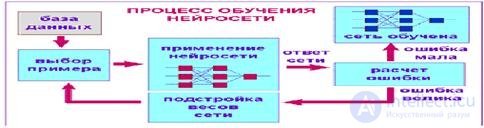
Fig.1.3 The process of learning the neural network
Based on the above, we can conclude that a network with back propagation is most suitable for solving forecasting problems. It allows you to formally train the network to predict the change in demand based on historical data about the requirement. The process of applying a neural network is shown in Figure 1.4.

Fig.1.4 The process of applying a neural network
For the description of algorithms and devices in neuroinformatics, a special "circuit design" has been developed, in which elementary devices - adders, synapses, neurons, etc. unite in networks designed to solve problems.
The most deserved and probably the most important element of neural systems is the adaptive adder. The adaptive adder calculates the scalar product of the input signal vector x by the parameter vector a. In the diagrams we will designate it as shown in Fig. 1.5. Adaptive call it because of the presence of the vector of adjustable parameters a. For many problems, it is useful to have a linear non-uniform function of the output signals. Its calculation can also be represented using an adaptive adder having n + 1 input and receiving a constant single signal at the 0th input (Fig. 1.6).
The nonlinear signal converter is depicted in Figure 1.7. It receives the scalar input signal x and translates it into j (x).
The branch point serves for sending one signal to several addresses (Fig. 1.8). It receives a scalar input x and transmits it to all its outputs.


Fig. 1.5. Adaptive adder. Fig. 1.6. Non-uniform adaptive adder.
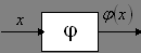

Fig.1.7 Nonlinear signal converter

Fig.1.8 Branch point

Fig.1.9 Formal neuron Fig.1.10 Linear communication (synapse)
Elements of layered and fully connected networks can be selected in different ways. There is, however, a standard choice - a neuron with an adaptive inhomogeneous linear adder at the input (Fig. 1.9).
Linear communication - synapse - is not found separately from adders, however, for some reasoning it is convenient to select this element (Fig. 1.1). It multiplies the input x by the “synapse weight” a.
The weights of the network synapses form a set of adaptive parameters, by tuning which, the neural network is trained to solve the problem. Usually, some restrictions are imposed on the range of changes in the weights of synapses, for example, the belonging of the synapse weight to the range [-1,1].
Among the entire multitude of neural network architectures, two basic architectures can be distinguished - layered and fully connected networks.
Layered networks: neurons are located in several layers (Fig. 1.1.11). The neurons of the first layer receive input signals, transform them and transfer them to the neurons of the second layer through branch points. Then the second layer works, etc. to the k-th layer, which produces output signals. Unless otherwise stated, each output signal of the i-th layer is fed to the input of all neurons i + 1-th. The number of neurons in each layer can be any and is not related in any way to the number of neurons in other layers. The standard way to input signals: each neuron of the first layer receives all input signals. Three-layer networks in which each layer has its own name are especially widespread: the first is the input, the second is hidden, the third is the output.

Fig.1.11 Layered network
Fully connected networks: have one layer of neurons; each neuron transmits its output to the rest of the neurons, including itself. The output signals of the network can be all or some of the output signals of neurons after several cycles of network operation. All input signals are given to all neurons.
There are two classes of tasks solved by the trained neural networks. These are the tasks of prediction and classification.
The tasks of prediction or forecasting are, in essence, the tasks of constructing a regression dependence of the output data on the input data. Neural networks can effectively build highly non-linear regression dependencies. The specificity here is such that, since mostly non-formalized tasks are solved, the user is primarily interested not in building a clear and theoretically justified relationship, but in obtaining a predictor device. The forecast of such a device will not directly go into action - the user will evaluate the output signal of the neural network based on his knowledge and form his own expert opinion. The exceptions are situations, based on the trained neural network create a control device for the technical system.
When solving classification problems, a neural network builds a dividing surface in the attribute space, and the decision on whether a particular class belongs to a particular class is made by an independent, network-independent device — the interpreter of the network response. The simplest interpreter arises in the problem of binary classification (classification into two classes). In this case, one output signal of the network is sufficient, and the interpreter, for example, relates the situation to the first class if the output signal is less than zero and to the second if it is greater than or equal to zero.
Classification into several classes requires interpreter complexity. The "winner takes all" interpreter is widely used, where the number of network output signals is equal to the number of classes, and the class number will correspond to the maximum output signal number.
One neural network can simultaneously predict several numbers, or simultaneously solve tasks and forecasting and classification. The need for the latter arises, however, extremely rarely, and it is better to solve different types of tasks by separate neural networks.
In the literature there are a significant number of features that a task must have in order for the use of neural networks to be justified and the neural network could solve it:
there is no algorithm or no principles for solving problems are known, but a sufficient number of examples have been accumulated;
the problem is characterized by large amounts of input information;
data is incomplete or redundant, noisy, partly contradictory.
Thus, neural networks are well suited for pattern recognition and solving classification, optimization, and forecasting problems.

Comments
To leave a comment
Approaches and directions for creating Artificial Intelligence
Terms: Approaches and directions for creating Artificial Intelligence