math programming

Optimization - in mathematics, computer science and operations research the problem of finding an extremum (minimum or maximum) of an objective function in a certain region of a finite-dimensional vector space bounded by a set of linear and / or nonlinear equalities and / or inequalities.

The theory and methods for solving an optimization problem are studying mathematical programming .

Mathematical programming is a field of mathematics that develops theory, numerical methods for solving multidimensional problems with constraints. In contrast to classical mathematics, mathematical programming deals with mathematical methods for solving problems of finding the best options from all possible.

Formulation of the optimization problem

In the design process, the usual task is to determine the best, in a sense, structure or parameter values ​​of the objects. Such a task is called optimization. If the optimization is associated with the calculation of the optimal values ​​of the parameters for a given object structure, then it is called parametric optimization . The task of choosing the optimal structure is a structural optimization .

A standard mathematical optimization problem is formulated in this way. Among the elements χ forming the set Χ, find an element χ ^* that delivers the minimum value f (χ ^* ) of a given function f (χ). In order to correctly set the optimization problem, you must specify:

1. Allowable set - set ;
2. Target function - display ;
3. Search criteria (max or min).

Then solve the problem 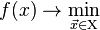means one of:

1. Show what .
2. Show that the objective function not limited to the bottom.
3. To find .
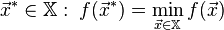4. If a then find .

If the minimized function is not convex, it is often limited to finding local minima and maxima: points such that everywhere in some of their neighborhoods for minimum and for the maximum.

If admissible set , then such a task is called an unconditional optimization problem , otherwise it is called a conditional optimization task .

Classification of optimization methods

The general record of optimization tasks sets a wide variety of their classes. The selection of the method depends on the class of the task (the effectiveness of its solution). The classification of tasks is determined by: the objective function and the admissible region (defined by a system of inequalities and equalities or by a more complex algorithm). ^[2]

Optimization methods are classified according to optimization tasks:

• Local methods: converge to some local extremum of the objective function. In the case of a unimodal objective function, this extremum is unique, and will be a global maximum / minimum.
• Global methods: deal with multi-extremal objective functions. In a global search, the main task is to identify trends in the global behavior of the target function.

The current search methods can be divided into three large groups:

1. deterministic;
2. random (stochastic);
3. combined.

By the criterion of the dimension of an admissible set, optimization methods are divided into one-dimensional optimization methods and multi -dimensional optimization methods.

By the form of the objective function and the admissible set, the optimization problems and the methods for their solution can be divided into the following classes:

• Optimization tasks in which the objective function and limitations are linear functions, resolved by the so-called linear programming methods.
• Otherwise, they deal with the problem of nonlinear programming and apply the appropriate methods. In turn, they are divided into two particular tasks:
  • if a and - convex functions, such a task is called a convex programming problem;
  • if a , then they deal with the problem of integer (discrete) programming .

According to the requirements for smoothness and the presence of partial derivatives in the objective function, they can also be divided into:

• direct methods requiring only calculations of the objective function at the points of approximation;
• first-order methods: require the calculation of the first partial derivatives of a function;
• second-order methods: they require the computation of the second partial derivatives, that is, the Hessian of the objective function.

In addition, optimization methods are divided into the following groups:

• analytical methods (for example, the Lagrange multipliers method and the Karush-Kuhn-Tucker conditions);
• numerical methods;
• graphic methods.

Depending on the nature of the set X , mathematical programming tasks are classified as:

• discrete programming problems (or combinatorial optimization) - if X is finite or countable;
• integer programming problems — if X is a subset of the set of integers;
• non-linear programming problems if the constraints or the objective function contain non-linear functions and X is a subset of finite-dimensional vector space.
• If all constraints and the objective function contain only linear functions, then this is a linear programming problem.

In addition, the sections of mathematical programming are parametric programming, dynamic programming and stochastic programming.

Mathematical programming is used in solving optimization problems of operations research.

The way of finding the extremum is completely determined by the class of the problem. But before you get a mathematical model, you need to perform 4 stages of modeling:

• Defining the boundaries of the optimization system
  • We reject those connections of the optimization object with the outside world that cannot greatly affect the result of the optimization, or, more precisely, those without which the solution is simplified.
• Selection of controlled variables
  • We “freeze” the values ​​of some variables (unmanaged variables). Others are left to accept any values ​​from the range of feasible solutions (controlled variables)
• Definition of constraints on managed variables
  • ... (equality and / or inequality)
• Selection of a numerical optimization criterion (for example, a performance indicator)
  • Create target function

Story

The problems of linear programming were the first thoroughly studied problems of searching for extremum of functions in the presence of inequality constraints. In 1820, Fourier and then in 1947 Danzig proposed a method of directional search of adjacent vertices in the direction of increasing the objective function — the simplex method, which became the main one in solving linear programming problems.

The presence of the term “programming” in the title of the discipline is explained by the fact that the first studies and the first applications of linear optimization problems were in the field of economics, since in English the word “programming” means planning, drawing up plans or programs. It is quite natural that the terminology reflects the close connection that exists between the mathematical formulation of the problem and its economic interpretation (the study of the optimal economic program). The term “linear programming” was proposed by Danzig in 1949 to study theoretical and algorithmic problems related to the optimization of linear functions under linear constraints.

Therefore, the name “mathematical programming” is connected with the fact that the goal of solving problems is to choose the optimal program of actions.

The selection of a class of extremal problems defined by a linear functional on a set defined by linear constraints should be attributed to the 1930s. One of the first to study the linear programming problem in general form was: John von Neumann, a mathematician and physicist, who proved the basic theorem on matrix games and studied the economic model bearing his name, and Kantorovich, a Soviet academician, a Nobel Prize winner (1975), formulated a series of linear programming problems and proposed in 1939 a method for solving them (the method of resolving factors), slightly different from the simplex method.

In 1931, the Hungarian mathematician B. Egervari considered a mathematical formulation and solved a linear programming problem called the “choice problem”, the solution method was called the “Hungarian method”.

Kantorovich together with M.K. Gavurin in 1949 developed the method of potentials, which is used in solving transport problems. Subsequent works of Kantorovich, Nemchinov, V. V. Novozhilov, A. L. Lurje, A. Brudno, Aganbegyan, D. B. Yudin, E. G. Golstein and other mathematicians and economists were further developed as a mathematical theory of linear and non-linear programming and application of its methods to the study of various economic problems.

Linear programming techniques are devoted to many works of foreign scientists. In 1941, F. L. Hitchcock set the transport task. The main method for solving linear programming problems, the simplex method, was published in 1949 by Danzig. Methods of linear and nonlinear programming were further developed in the works of Kuhn ( Eng. ), A. Tucker ( Eng. ), Gass (Saul. I. Gass), Charnes (Charnes A.), Beale EM, and others.

Simultaneously with the development of linear programming, much attention was paid to nonlinear programming problems in which either the objective function, or the constraints, or both are nonlinear. In 1951, the paper by Kuhn and Tucker was published, in which the necessary and sufficient conditions for optimality for solving nonlinear programming problems are given. This work served as the basis for further research in this area.

Since 1955, many works have been published on quadratic programming (the work of Beal, Barankin and Dorfman R., Frank M. and Wolfe P., Markowitz, and others). The work of Dennis (Dennis JB), Rosen (Rosen JB) and Zontendijk (Zontendijk G.) developed gradient methods for solving nonlinear programming problems.

Currently, for the effective application of mathematical programming methods and problem solving on computers, algebraic modeling languages ​​have been developed, representatives of which are AMPL and LINGO.