Lecture
Differential evolution (born differential evolution) is a multidimensional mathematical optimization method that belongs to the class of stochastic optimization algorithms (that is, it works using random numbers) and uses some ideas from genetic algorithms.
This is a direct optimization method, that is, it requires only the ability to calculate the values of the target functions, but not its derivatives. The method of differential evolution is designed to find a global minimum (or maximum) of non-differentiable, non-linear, multimodal (having, possibly, a large number of local extremes) functions of many variables. The method is simple to implement and use (contains few control parameters that require matching), easily parallelized.
The method of differential evolution was developed by Rainer Storn and Kenneth Price, first published by them in 1995 [1] and developed further in their later works. [2] [3]
Algorithm
In its basic form, the algorithm can be described as follows. Initially, a number of vectors are generated, called generation. The vectors are the points of the n-dimensional space in which the objective function f (x) is defined, which is to be minimized. At each iteration, the algorithm generates a new generation of vectors, randomly combining vectors from the previous generation. The number of vectors in each generation is the same and is one of the parameters of the method.
A new generation of vectors is generated as follows. For each vector x_i from the old generation, three different random vectors v_1, v_2, v_3 are selected from among the vectors of the old generation, except for the vector x_i itself, and the so-called mutant vector is generated using the formula:
v = v_1 + F \ cdot (v_2 - v_3),
where F is one of the parameters of the method, some positive real constant in the interval [0, 2].
Over the mutant vector v, a crossover operation is performed, consisting in that some of its coordinates are replaced by corresponding coordinates from the original vector x_i (each coordinate is replaced with a certain probability, which is also one of the parameters of this method). The vector obtained after crossing is called a trial vector. If it turns out to be better than the vector x_i (that is, the value of the objective function has become less), then in the new generation the vector x_i is replaced with the test vector, and otherwise x_i remains.
Examples of practical applications
The Yandex search engine uses the differential evolution method to improve its ranking algorithms. [4] [5]
At Habré there are many articles on evolutionary algorithms in general and genetic algorithms in particular. In such articles, the general structure and ideology of a genetic algorithm is usually described in more or less detail, and then an example of its use is given. Each such example includes some chosen variant of the procedure of crossing individuals, mutations and selection, and in most cases for each new task one has to invent his own version of these procedures. By the way, even the choice of representing the element of the decision space by the gene vector greatly influences the quality of the resulting algorithm and is essentially an art.
At the same time, many practical problems can easily be reduced to an optimization problem of finding the minimum of the function n real variables, and for such a typical variant I would like to have a ready-made reliable genetic algorithm. Since even the definition of crossing operators and mutations for vectors consisting of real numbers is not entirely trivial, then “making” a new algorithm for each such task turns out to be particularly time-consuming.
Under the cat is a brief description of one of the most well-known genetic algorithms of real optimization - the algorithm of differential evolution (Differential Evolution, DE). For complex problems of optimizing the function of n variables, this algorithm has such good properties that it can often be considered as a ready-made “building block” when solving many problems of identification and pattern recognition.
I will assume that the reader is familiar with the basic concepts used in the description of genetic algorithms, so I will go straight to the point, and in conclusion I will describe the most important properties of the DE algorithm.
Generation of the initial population
A random set of N vectors from the space R n is selected as the initial population. The distribution of the initial population should be selected on the basis of the characteristics of the optimization problem to be solved - usually a sample of n -dimensional uniform or normal distribution is used with the specified expectation and variance.
Reproduction of descendants
At the next step of the algorithm, each individual X from the initial population is crossed with a randomly selected individual C , different from X. The coordinates of vectors X and C are considered as genetic traits. Before crossing, a special mutation operator is used — not the original, but the distorted genetic characteristics of the individual C are involved in the crossing:

Here, A and B are randomly selected members of the population, distinct from X and C. The parameter F defines so-called. mutation force - the amplitude of the disturbances introduced into the vector by external noise. It should be particularly noted that, as noise that distorts the “gene pool” of the individual C , it is not the external source of entropy that is used, but the internal one — the difference between randomly selected representatives of the population. Below we will focus on this feature in more detail.
Crossing is as follows. It sets the probability P , from which the descendant T inherits the next (mutated) genetic trait from the parent C. The corresponding attribute from parent X is inherited with probability 1 - P. In fact, a binary random variable with mathematical expectation P is played n times, and for its single values, the inheritance (transfer) of a distorted genetic trait from parent C (that is, the corresponding coordinates of vector C ' ) is performed, and for zero values, the genetic trait is inherited from parent X. As a result, a descendant vector T is formed .
Selection
The selection is carried out at each step of the functioning of the algorithm. After the formation of the descendant vector T , the objective function is compared for it and for its “direct” parent X. The new population is transferred to the one of the vectors X and T , on which the objective function reaches a smaller value (we are talking about the minimization problem). It should be noted here that the described selection rule guarantees the invariance of the population size during the operation of the algorithm.
Discussion features of the algorithm DE
In general, the DE algorithm is one of the possible "continuous" modifications of the standard genetic algorithm. At the same time, this algorithm has one significant feature, which largely determines its properties. The DE algorithm does not use an external random number generator as a noise source, but an “internal” one, implemented as the difference between randomly selected vectors of the current population. Recall that a set of random points selected from a certain general distribution is used as the initial population. At each step, the population is transformed by some rules and as a result, in the next step, a set of random points is again used as a source of noise, but some new distribution law corresponds to these points. Experiments show that, in general, the evolution of a population corresponds to the dynamics of a “swarm of midges” (ie, a random cloud of points) moving as a whole along the relief of an optimized function, repeating its characteristic features. In the case of falling into a ravine, the cloud takes the form of this ravine and the distribution of points becomes such that the expectation of the difference of two random vectors is directed along the long side of the ravine. This ensures fast movement along narrow elongated ravines, whereas gradient methods under similar conditions are characterized by the dynamic dynamics “from wall to wall”. These heuristic considerations illustrate the most important and attractive feature of the DE algorithm — the ability to dynamically model the features of the relief of an optimized function, adjusting the distribution of the “built-in” noise source to them. This explains the remarkable ability of the algorithm to quickly pass complex ravines, ensuring efficiency even in the case of complex terrain.
Parameter selection
For population size N , the value Q * n is usually recommended, where 5 <= Q <= 10 .
For the mutation force F, reasonable values are chosen from the segment [0.4, 1.0] , with a good initial value being 0.5 , but with a rapid degeneration of the population far from the solution, the parameter F should be increased.
The probability of mutation P varies from 0.0 to 1.0 , and you should start with relatively large values ( 0.9 or even 1.0 ) to test the possibility of quickly obtaining a solution by random search. Then, the parameter values should be reduced to 0.1 or even 0.0 , when there is practically no variation in the population and the search turns out to be convergent.
Convergence is most affected by population size and mutational strength, and the probability of mutation serves to fine tune it.
Numerical example
The features of the DE method are well illustrated when it is run on the standard test function of Rosenbrock

This function has an obvious minimum at the point x = y = 1 , which lies at the bottom of a long winding ravine with steep walls and a very flat bottom.
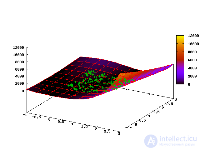
When running with a uniform initial distribution of 200 points per square [0, 2] x [0, 2] after 15 steps, we get the following distribution of the population:
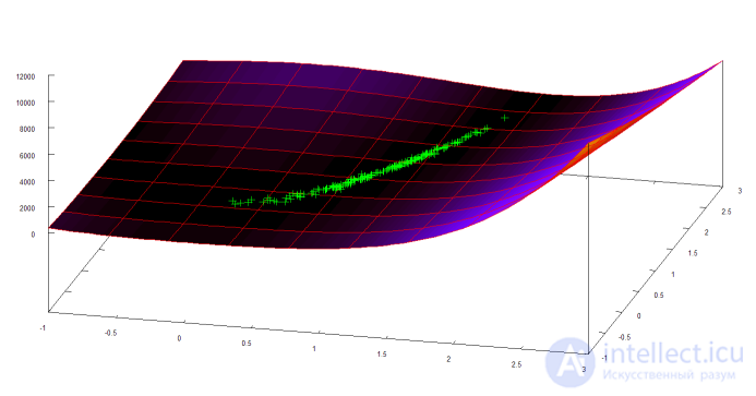
It can be seen that the “cloud” of points is located along the bottom of the ravine and most mutations will lead to a shift of points also along the bottom of the ravine, i.e. the method adapts well to the peculiarities of the geometry of the solution space.
The following animated picture shows the evolution of the point cloud in the first 35 steps of the algorithm (the first frame corresponds to the initial uniform distribution):
Links

Comments
To leave a comment
Evolutionary algorithms
Terms: Evolutionary algorithms